The Potential Transformer Replacement: Mamba

Transformer models and their components are behind many artificial intelligence (AI) breakthroughs. While they dominate, their quadratic complexity limits efficiency on long sequences. Various subquadratic-time models, such as linear attention, gated convolutions, and structured state space models (SSMs), have emerged to tackle this problem. However, these models often struggle with discrete, content-rich data like text.

Last year, a new architecture called Mamba emerged to address such problems. This architecture matches Transformer performance while scaling linearly in sequence length, offering a powerful alternative for efficiently handling large-scale data.

In this article, we will explore Mamba, covering:

• Key concepts needed to understand Mamba.

• The fundamental architecture of Mamba.

• A detailed overview of how Mamba works.

• A comparison with Transformers, examining Mamba's performance relative to traditional models.

If you want to explore more details, here is the Mamba Paper.

The Problem with Transformers

Transformer architecture has been a game-changer, especially because of the self-attention mechanism. It allows transform-based models to simultaneously consider all tokens in a sequence, making them practical for tasks requiring long-range dependencies. This is why they are so effective in generating a long essay coherently. So, why do we require a new architecture like Mamba?

To understand why, let’s briefly revisit the core elements of the Transformer architecture. Transformers treat input data, like text, as a sequence of tokens. The significant advantage is that each token can "attend" to any other token in the sequence. This is achieved through self-attention, which creates a matrix comparing the relevance of each token to every other token in the sequence. During training, this process is performed in parallel, allowing fast training and efficient representation learning.

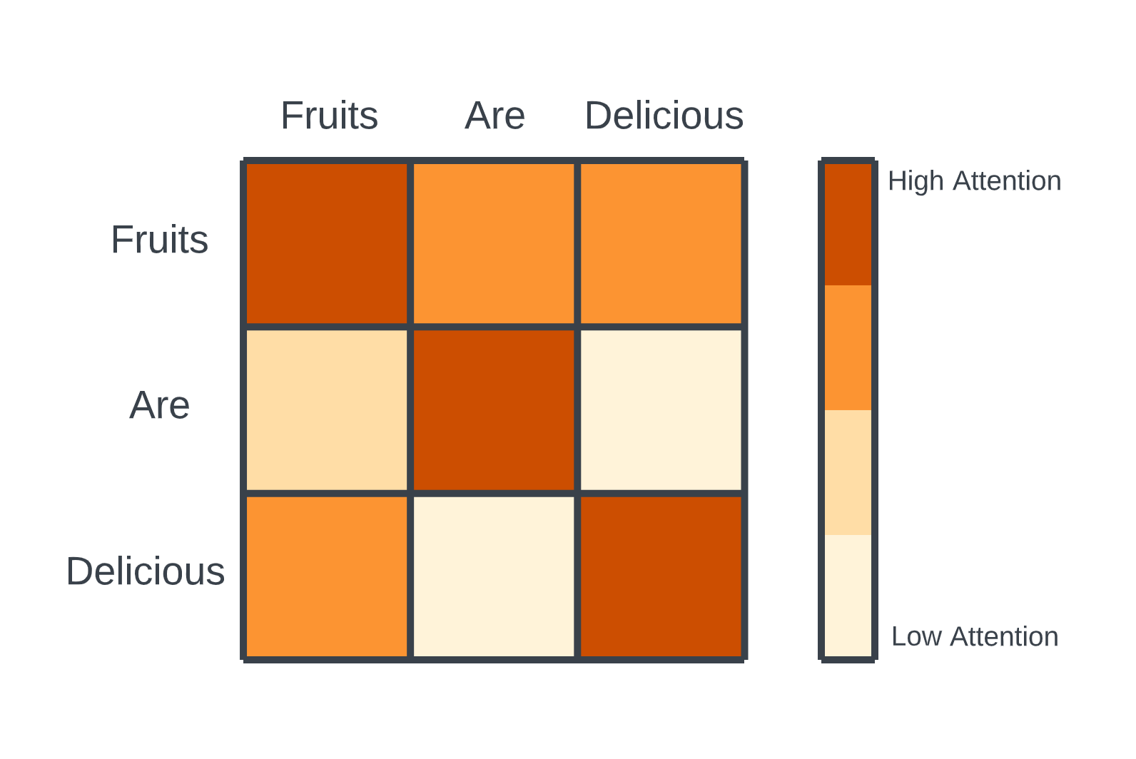Attention Mechanism in Transformers.png

Attention Mechanism in Transformers | Source

However, the self-attention mechanism has a critical drawback during inference (generating new text or tokens). At each step, the model must recompute the attention matrix for the entire sequence, even for previously generated tokens. This results in quadratic time complexity, where generating tokens for a sequence of length requires computations. As the sequence length grows, the computational and memory demands become unsustainable, creating a significant bottleneck.

Recurrent Neural Networks

Recurrent Neural Networks (RNNs) offered a partial solution in the past. Unlike Transformers, RNNs maintained a state (latent information), allowing them to process sequences step-by-step without recomputing the entire sequence for each token. However, RNNs struggled to capture long-range dependencies effectively and were eventually outperformed by Transformers.

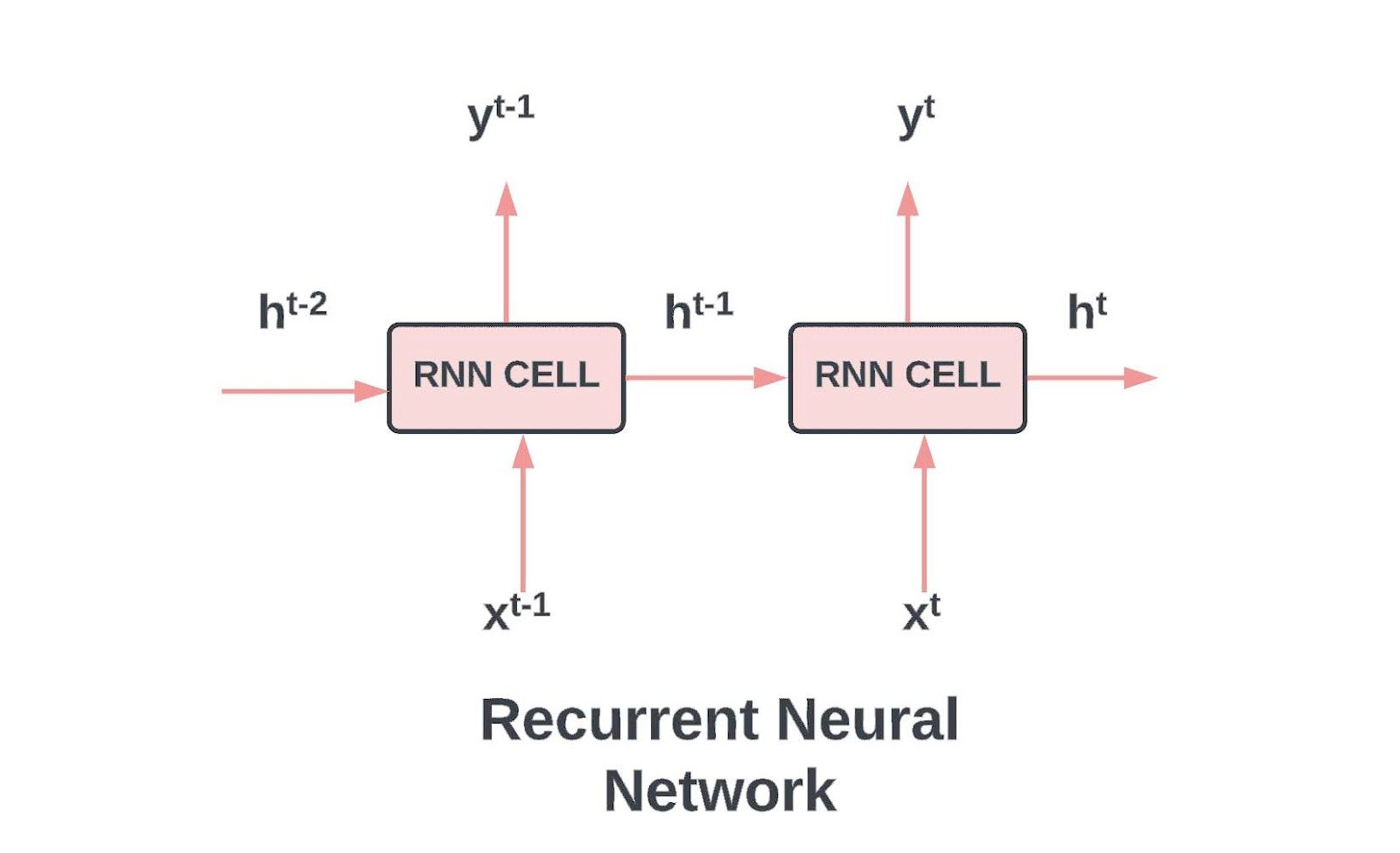RNN’s cell takes two inputs.jpg

RNN’s cell takes two inputs: the current input $X$ and the previous hidden state $H$ | Source

Mamba combines the strengths of both Transformers and RNNs by capturing long-range dependencies while maintaining a manageable complexity of time. But first, let's explore the State Space Model, as Mamba is built upon this foundation.

Key Concepts that Build up to Mamba

To learn the Mamba hierarchy, we need to have a solid understanding of key concepts.

State Space Model

A State Space Model (SSM) represents and understands how systems change over time. It describes dynamic systems, like moving objects or signals, by focusing on their current state and how they respond to inputs.

Core Concepts of SSMs:

• State Space: Think of the state space as a map of all possible positions a system can be in. For example, if you’re navigating through a maze, each point on the map represents a specific location.

• State Vectors: These are like coordinates that describe where you are on the map. They can include details like your current position and distance from the exit. In language models, similar vectors help explain the "state" of an input sequence. These can be thought of as embeddings.

How SSMs Work:

At any given time $t$, an SSM works like this:

• Input Sequence $x(t)$: This information you provide to the model, like a command to move left in the maze.

• Latent State Representation $h(t)$: This is the updated "knowledge" about the system's current state. It captures important information, such as your position and how to get to the exit.

• Predicted Output Sequence $y(t)$: This tells you what the system will do next, suggesting you move left again to reach the exit faster.

SSMs use two main equations to track changes:

1. State Equation: This equation shows how the current state changes based on the input:

$h'(t)=Ah(t)+Bx(t)$

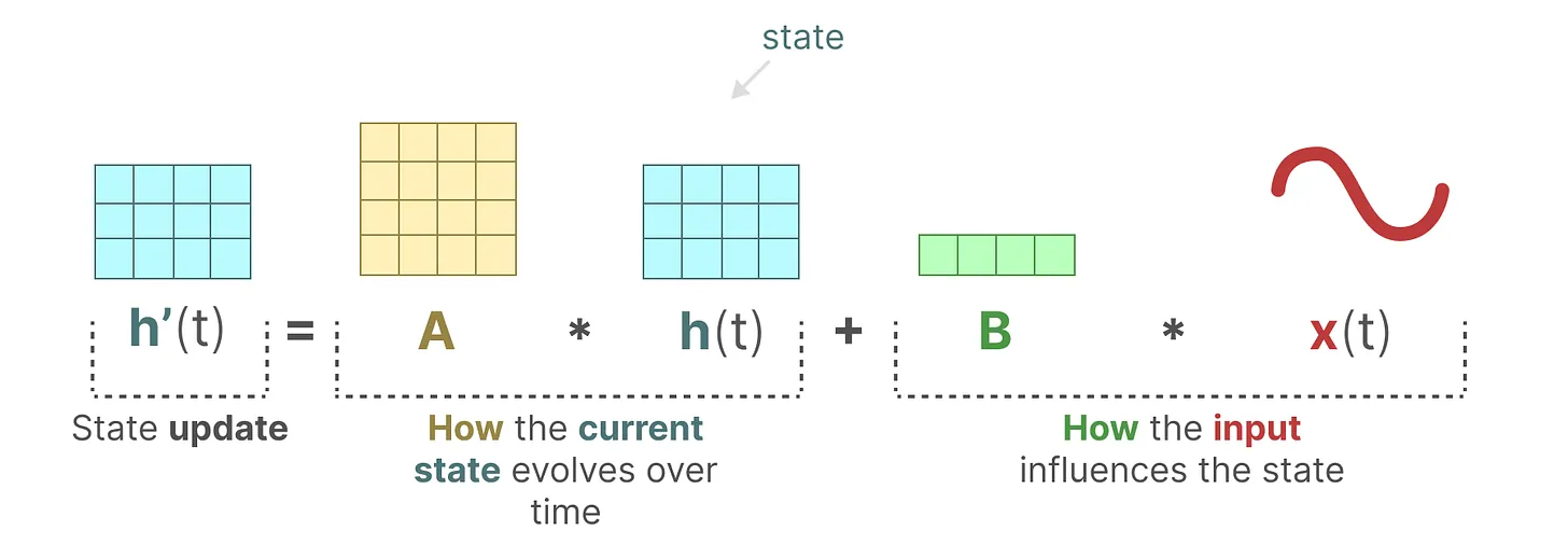State Equation of the State Space Model.png

State Equation of the State Space Model | Source

• Matrix $A$: This matrix tells how different parts of the system connect. Matrix $A$ in SSMs is crucial for retaining past information and determining how much history is captured in the hidden state. Using HiPPO (High-order Polynomial Projection Operators), matrix $A$ compresses input signals, effectively capturing recent tokens while decaying older ones.

• Matrix $B$: This shows how the input affects the current state.

2. Output Equation: This equation explains how the state leads to an output:

$y(t)=Ch(t)+Dx(t)$

Output Equation of the State Space Model.png

Output Equation of the State Space Model | Source

• Matrix $C$: This translates the state into an output.

• Matrix $D$: This provides a direct path from the input to the output, similar to a shortcut. That’s why it is also referred to as a skip connection.

The matrices $A$, $B$, $C$, and $D$ are often referred to as parameters because they are learnable components of the model.

These equations help SSMs predict what will happen next based on what they’ve learned from the input. This approach is helpful for modeling systems that change continuously over time, like tracking movements or signals.

Here’s what the architecture looks like:

The Complete Architecture of SSM.png

The Complete Architecture of SSM | Source

The equations are continuous, as they depend on time, whereas large language models process input as discrete text. Let's explore how to convert a continuous signal into a discrete signal.

Discretization

Since most inputs we encounter, like textual sequences, are discrete, we need a way to convert our continuous model into a discrete one. We use the Zero-order hold technique to transform a continuous signal into a discrete one. Here’s how it works:

• Holding Values: Each time we receive a discrete input, we have its value until we receive the next one. This process effectively creates a continuous signal that the SSM can utilize.

• Step Size $\Delta$ : The duration we hold the value is controlled by a learnable parameter called the step size $\Delta$. This parameter represents the input's resolution and dictates how finely we sample the continuous signal.

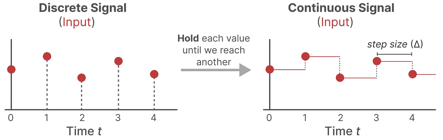Zero-Order Hold Technique for Discretization.png

Zero-Order Hold Technique for Discretization | Source

Once we have this continuous representation of our input, we can generate outputs in a similar constant form and then sample these values according to the input's time steps. The sampled values become our discretized output.

With these, our matrices are represented differently:

$\bar{A}=exp(\Delta{A})$

$\bar{A}=(\Delta{A})^{-1}(exp(\Delta{A})-I)·\Delta{B}$

These matrices are now suitable for our language tasks. Here are how the state and output equations will look like:

State equation $H_{k}=Ah_{k-1}+Bx_k$

Output equation $y_{k}=Ch_{k}+Dx_{k}$

We use $k$ instead of $t$ to denote discretized time steps, which makes the differences between continuous and discrete SSMs more apparent.

Recurrent and Convolutional Representations in State Space Models (SSMs)

When working with State Space Models (SSMs), we can represent them in multiple ways depending on the task and the form of input data. Two common representations that help compute SSMs are Recurrent Representation and Convolution Representation.

The Recurrent Representation

This approach aligns with the way Recurrent Neural Networks (RNNs) handle sequences. By breaking continuous signals into discrete timesteps, we can calculate how each input influences the system step by step. At each timestep $k$, we determine how the current input $Bx_k$ interacts with the previous state $Ah_{k-1}$, which updates the state, allowing us to predict the following output $Ch_k$.

This method is similar to RNNs because it processes sequences iteratively, using the prior state at every step. This unrolling of the sequence over time mirrors the process in RNNs, where past information influences current predictions. It offers a structured, step-by-step method for sequential data processing.

The Convolution Representation

Another way to represent SSMs is through a convolutional approach, commonly used in image recognition tasks but also applicable to sequences. Instead of processing each input individually at every timestep, we apply a filter, or kernel, over the sequence of tokens, aggregating features across the input in one-dimensional space.

This method resembles Convolutional Neural Networks (CNNs), where the kernel moves across the input sequence, performing calculations at each position. This approach can be trained in parallel, similar to how CNNs work with image data, making it computationally efficient for training. However, during inference, the fixed size of the kernel limits its flexibility compared to the recurrent method.

Combining Together

Recurrent and convolutional representations offer unique advantages. The recurrent SSM allows for efficient inference, while the convolutional SSM supports parallelized training. Combining these allows us to use the convolutional representation for faster training and the recurrent representation for more efficient inference.

However, a key limitation of these models is Linear Time Invariance (LTI), where the matrices $A$, $B$, and $C$ remain fixed across all timesteps, leading to a static, content-agnostic representation. This is where Mamba introduces improvements to make the system more dynamic and adaptive.

What is Mamba and How Mamba Works?

Mamba is a new architecture for sequence modeling, designed to offer an alternative to the Transformer models commonly used in machine learning, especially for handling long sequences of data. It introduces a Selective State Space Model (SSM), which allows the model to process information more efficiently by focusing on relevant data and discarding irrelevant parts.

Mamba can address the following issues present in State Space Models (SSMs):

• Linear Time Invariance: SSMs treat each token in a sequence equally because the matrices (A, B, and C) are static and remain the same for every token, which limits their ability to adapt to different inputs dynamically.

• Poor Content-Awareness: Due to the fixed nature of these matrices, SSMs cannot focus on or ignore specific inputs based on the content, making them ineffective at performing content-aware reasoning.

• Inability to Recall Patterns: In tasks of reproducing patterns, SSMs struggle to recall specific tokens from their history due to their time-invariant nature. As Matrix B remains independent of the input, it prevents the model from adapting to particular inputs and recognizing patterns within the sequence.

Here’s how Mamba solves it:

Selective Scan Algorithm

• Dynamic Matrices (B and C): Unlike traditional state-space models, where the matrices are static, Mamba makes the matrices B and C dynamic and dependent on the input. This allows the model to focus on relevant information in the sequence and ignore irrelevant parts. This approach addresses the content-awareness problem of prior models like S4, enabling Mamba to perform well on tasks that require selective attention.

• Input-Adaptive Step Size: By incorporating an adjustable step size (∆), Mamba can compress input selectively. A significant step focuses more on input, while a minor step emphasizes prior context, balancing immediate input and long-term dependencies.

Hardware-Aware Algorithm

• Parallel Scan Algorithm: Recurrence in state space models typically limits parallelization because each state depends on the previous one. However, Mamba introduces a parallel scan mechanism that breaks this limitation, enabling efficient, hardware-accelerated parallel computation. This makes it scalable to longer sequences without suffering performance degradation.

• Kernel Fusion: By combining multiple operations into a kernel, Mamba reduces the need to store and transfer intermediate results between memory levels (such as DRAM and SRAM in GPUs). This optimizes memory access patterns, improving both speed and energy efficiency, especially on modern hardware like GPUs.

• Recomputation: Instead of storing intermediate states for backpropagation, Mamba recalculates them during the backward pass, reducing the memory burden. Though this seems computationally expensive, the savings in memory access time make it more efficient, especially for long sequences.

Enhanced Model Structure

Building on the above enhancements, here’s what the structure of the Mamba model looks like:

• Recurrent SSMs and Long-Range Dependencies: Mamba leverages the HiPPO (Highly Parallelizable Ordinary Differential Equation) initialization for matrix A to efficiently capture long-range dependencies, which is crucial for tasks like language generation.

• Stacking Mamba Blocks: Mamba blocks can be stacked similarly to transformer decoder blocks. Doing so allows them to process sequences more deeply, passing the output of one Mamba block into another.

• Normalization and Softmax Layers: These layers are added to the architecture to ensure smooth and stable training and to select appropriate output tokens, aligning with the architectures seen in transformers.

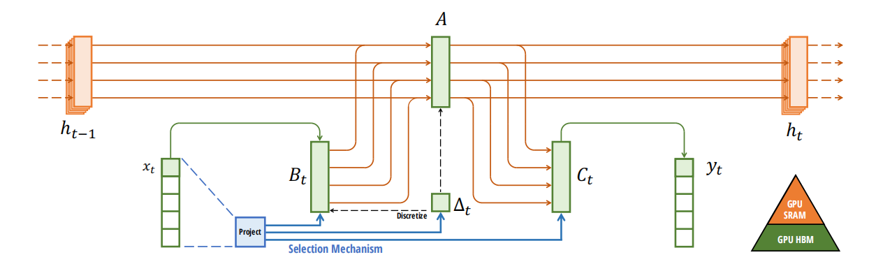The Selective SSM or Mamba Architecture.png

The Selective SSM or Mamba Architecture | Source

Let's now learn how it stacks up against the Transformer model.

Mamba vs Transformers

The Mamba architecture was evaluated against the standard Transformer model, specifically the GPT-3 architecture, and a more potent variant called Transformer++. The evaluation focused on pretraining metrics, such as perplexity and zero-shot performance on various downstream tasks.

1. Pretraining Performance

Mamba's pretraining was conducted using the Pile dataset, and the model sizes were set to mirror those of GPT-3. The scaling laws were analyzed under the Chinchilla protocol, revealing that Mamba outperformed the standard Transformer model, particularly in scenarios related to longer sequences. Mamba is the first attention-free model to match the advanced Transformer recipe (Transformer++) performance across model sizes ranging from approximately 125 million to 1.3 billion parameters. The results indicate that Mamba can perform similarly or better than Transformer models using fewer parameters.

2. Zero-Shot Evaluations

In a range of popular downstream tasks, Mamba consistently outperformed various open-source models, including Pythia and RWKV, which were trained using the same tokenizer and dataset. Mamba demonstrated best-in-class performance across all tasks in zero-shot evaluations, significantly surpassing Pythia and RWKV at comparable model sizes.

3. Model Efficiency

The Mamba architecture exhibited superior efficiency in both training and inference. During the benchmarks, Mamba achieved 4-5 times higher inference throughput than Transformers of similar sizes. The absence of key-value (KV) caching allowed Mamba to utilize larger batch sizes, enhancing its overall throughput.

4. Downstream Task Performance

In downstream tasks, such as language modeling and genomic sequence classification, Mamba showed a pronounced advantage in leveraging longer context lengths. The selective state space model (SSM) mechanism in Mamba maintained performance even with highly long sequences, while Transformer-based models experienced diminishing returns as context lengths increased.

5. Scalability and Adaptability

Mamba's architecture has shown promising scalability. Its performance improved consistently as model sizes increased, outperforming both HyenaDNA and Transformer++ models with significantly fewer parameters. Mamba’s selective SSM capabilities also enable it to adapt effectively to varying context lengths.

Conclusion

The article discusses how Mamba competes well with the Transformer model. To recap, we discussed:

• Transformers effectively manage long-range dependencies but face challenges with time complexity during inference.

• State Space Models (SSMs) provide a mathematical framework for representing dynamic systems and tracking state changes. They use two key equations: one for updating states and another for generating outputs.

• Discretization transforms continuous inputs into discrete representations for processing in SSMs. Recurrent and convolutional approaches, one for inference and the other for training, are used to compute SSMs.

• Mamba uses selective scan and hardware-aware algorithms to address the shortcomings and compare them well to the Transformer model.

Mamba offers a compelling solution to the challenges faced by traditional models like Transformers. Leveraging the principles of State Space Models, it balances efficiency and performance.

Additional Resources

Here are some further exploration resources:

• Scaling Laws for Neural Language Models

• Mamba: Linear-Time Sequence Modeling with Selective State Spaces

• HiPPO: Recurrent Memory with Optimal Polynomial Projections

• Long Range Arena: A Benchmark for Efficient Transformers

• Efficiently Modeling Long Sequences with Structured State Spaces

• Legendre Memory Units: Continuous-Time Representation

• Efficient Memory Management for Large Language Model Serving with PagedAttention

• What is RoBERTa?

• What are Vector Databases and How Do They Work?

• What is RAG?