Learn
AI & Machine Learning

Mastering BM25: A Deep Dive into the Algorithm and Its Application in Milvus

Mar 08, 202415 min read

We can easily implement the BM25 algorithm to turn a document and a query into a sparse vector with Milvus. Then, these sparse vectors can be used for vector search to find the most relevant documents according to a specific query.

By Ruben Winastwan

Read the entire series

Information retrieval algorithms are important in search engines to ensure the relevance of the search results to the user's query.

Imagine a use case where we're looking for research papers on a specific topic. When we write "RAG" as a keyword in a search engine, we obviously want to get a collection of papers that talk about different RAG methods instead of other general NLP methods. This is where information retrieval algorithms play their role. They ensure that we get papers that are highly relevant to our keyword.

There are two commonly applied algorithms for information retrieval: TF-IDF and BM25. In this article, we'll discuss everything about BM25. However, before we delve into it, it's best if we understand the fundamentals of TF-IDF first because BM25 is basically an extension of TF-IDF.

The Fundamental of TF-IDF

Term Frequency-Inverse Document Frequency (TF-IDF) is an information retrieval algorithm based on a statistical method. It measures the importance of a keyword within a document relative to a collection of documents.

As you can see from its name, TF-IDF consists of two components: Term Frequency (TF) and Inverse Document Frequency (IDF). They measure different aspects, but ultimately, we multiply the two components together to obtain the final score that estimates the relevance of a word within a document.

The TF component of traditional TF-IDF measures the occurrence of a particular keyword in a document.

The equation above is quite intuitive: the more instances of our keyword we find in a document, the higher the TF value will be.

On the other hand, the IDF component measures the proportion of documents in a collection that contain our keyword. In other words, this part informs us about how many documents our keyword appears in.

We can see that the more frequently our keyword appears across documents, the lower its IDF score becomes. This is because we want to penalize common words such as 'a', 'an', 'is', etc., as they tend to appear in many documents.

After computing the TF and IDF components, we multiply the results to obtain the final TF-IDF score of a keyword.

From the final equation above, we can see that TF-IDF captures the importance of a keyword by assigning it a higher score if it appears frequently in one document but rarely in others.

When given a user keyword or query, a search engine can use TF-IDF scores to measure the relevance between the keyword and the collection of documents. Then, the search engine can rank the documents and present the most relevant ones to the user.

Problems with TF-IDF

There are two problems with the TF-IDF formula that can be improved.

First, let’s say we have the word “rabbit” as a query and two documents to compare. In Document A, “rabbit” appears ten times, and that document has 1000 words. On the other hand, our keyword appears only once in document B, and that document has ten words.

Upon closer inspection, we can see the limitation of TF-IDF straight away. The TF score of document A would be 10, whilst the score of document B would be 1. Therefore, document A would be recommended to us compared to document B.

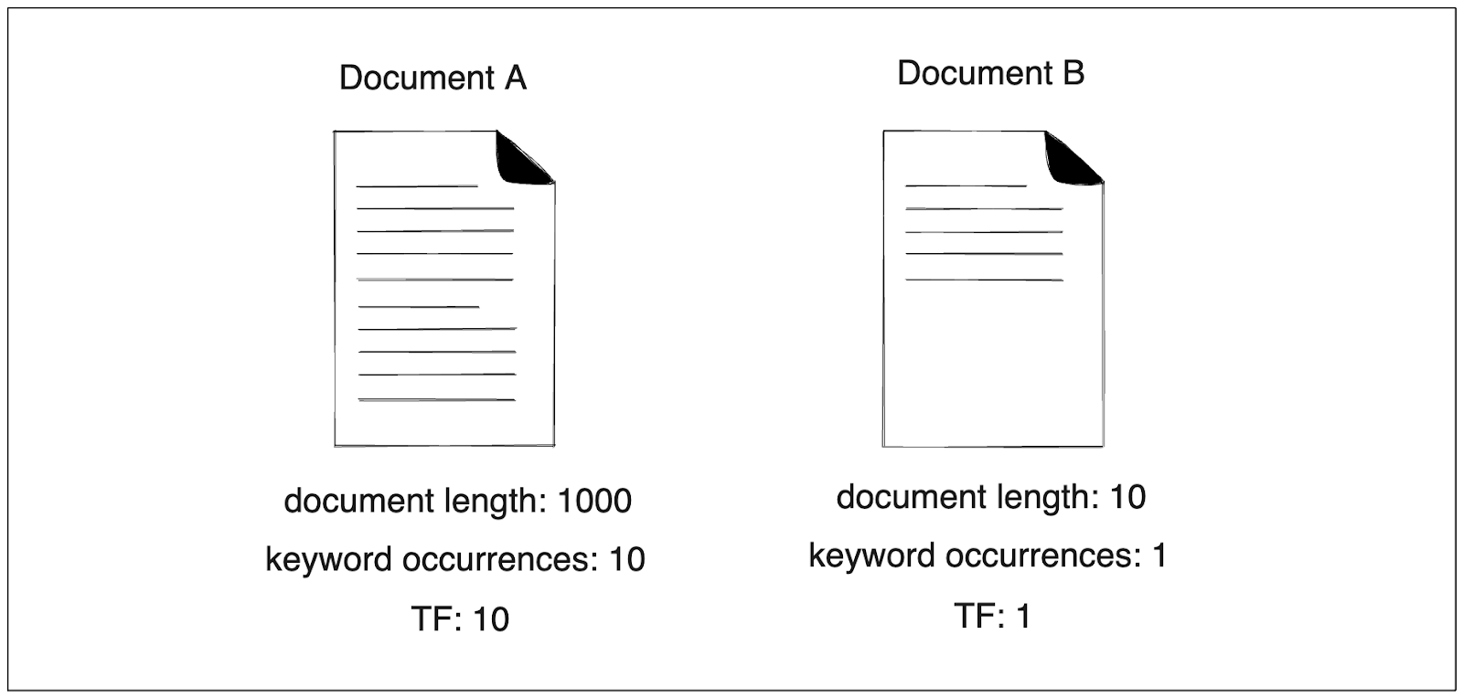Image by author

However, if we take document length into account, we might argue that we would prefer document B over document A.

When a document is very short and contains "rabbit" once, it's a more convincing indication that the document truly talks about a rabbit. Conversely, if a document has thousands of words and it mentions "rabbit" 10 times, we can't guarantee with certainty that the document talks specifically about a rabbit.

To address this issue, the normalized variant of TF-IDF divides TF by the document length. The TF equation of the TF part then looks like this:

But it still has one problem that needs to be optimized, which is related to keyword saturation.

If we take a look at the TF part of TF-IDF, the more we can find our keyword in a document, the higher the TF would be. The relationship is linear and this seems like a good thing, as we want to continuously reward a document that contains our keyword. However, if we find the keyword “rabbit” 400 times in a document, does that really mean that this document is twice as relevant as another document that contains only 200 occurrences?

We can argue that if the keyword “rabbit” occurs so many times in a document, we can say that this document is certainly relevant to our keyword. Additional occurrences of the keyword in this document shouldn’t increase the likelihood of its relevance in a linear scale.

The score jump caused by keyword occurrences in a document from 2 to 4 should have more impact than the jump from 200 to 400. And this is what is currently missing from the TF-IDF formula. 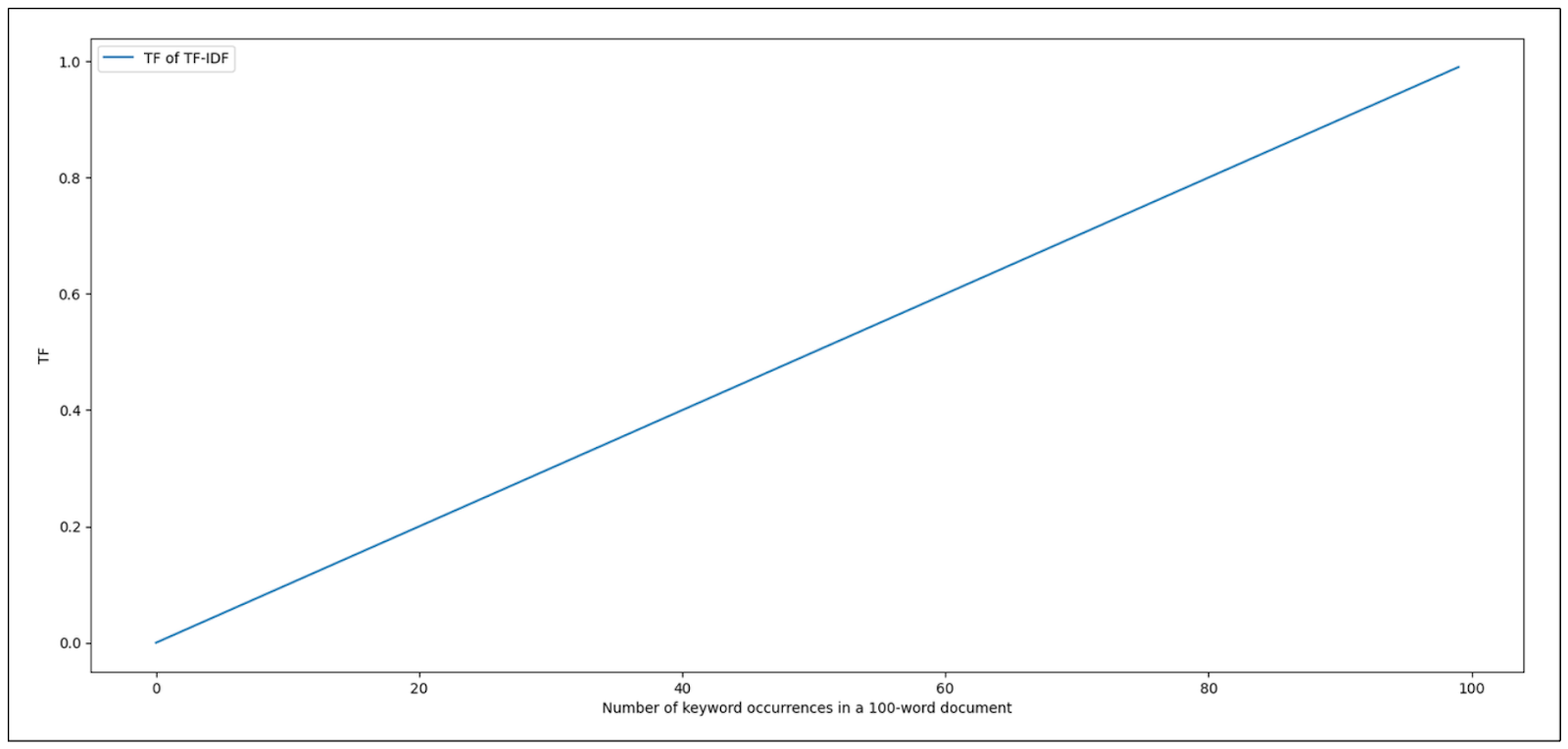Image by author

As you can see from the visualization above, given that we fixed the number of words in a document to 100, the TF score of TF-IDF increases linearly as the occurrence of our keyword increases.

So, how can we improve TF-IDF? This is where we need the BM25 algorithm.

The Fundamental of BM25

Best Matching 25 (BM25) is an algorithm that can be seen as an improvement to traditional TF-IDF by addressing all of its problems mentioned in the previous section.

Let’s discuss keyword saturation first. The TF part of TF-IDF will grow linearly as the number of occurrences of a keyword grows in a document. The score jump from 2 to 4 keywords will be identical to the jump from 50 to 52 keywords.

BM25 introduces a slightly different formula for the TF part compared to TF-IDF, and we’re going to slowly reveal each component one by one to make it easier for us to make sense of what happens under the hood.

First, instead of just relying on the number of occurrences of a keyword, BM25 introduces a new parameter in its TF equation:

The parameter k above acts as the parameter to control the contribution of each incremental occurrence of our keyword into the TF score. Let’s take a look at the visualization below to see the impact of k.

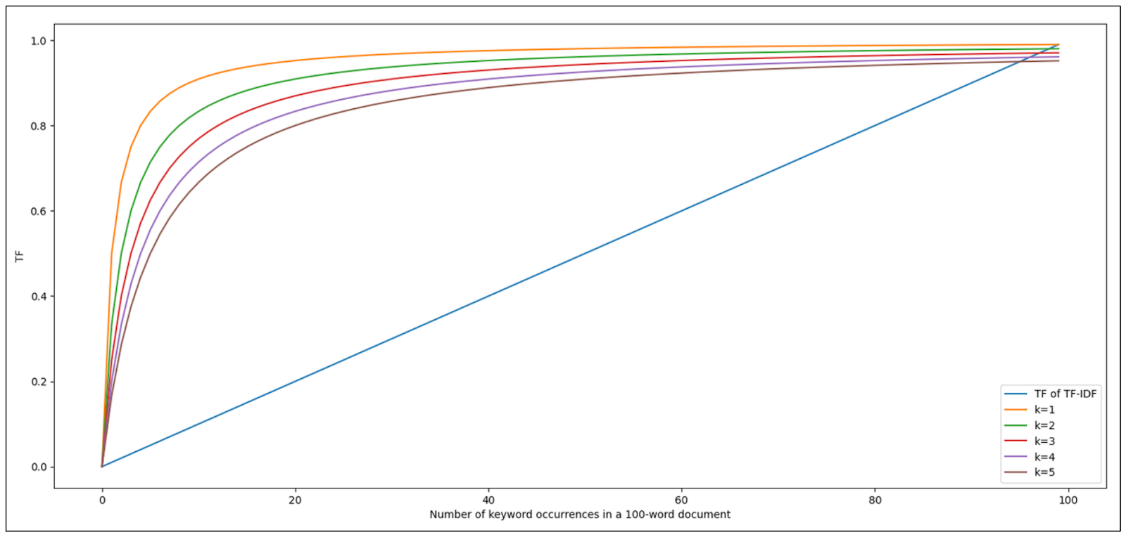Image by author

As you can see, the impact of the first few keyword occurrences to the overall TF score is big. However, as our keyword appears more and more in the document, its contribution to the overall TF score becomes more irrelevant. The higher the k value, the slower the contribution growth of each occurrence of our keyword to the TF score will be. This solves the drawback of TF-IDF related to keyword saturation.

Another fundamental improvement of BM25 compared to traditional TF-IDF is that BM25 takes the document length into account. With BM25, a 10-word document that contains one keyword would be a stronger candidate than a 1000-word document that contains 10 keywords.

The term $|D|$ represents the document length, while avg(D) represents the average length of documents in our corpus. You can already see the impact of this document normalization on our k parameter. If the document is shorter than average, the value of TF/(TF+k) will increase, and vice versa. In other words, shorter documents will approach the saturation point quicker than longer documents.

However, we can’t treat all corpora the same way. In some corpora, the length of the documents matters a lot, while in others, the length of the documents is not important at all. Therefore, an additional parameter b is introduced in the TF equation to control the importance of document length in the overall score.

We can see that if we set the value of b to 0, then the ratio D/avgD wouldn’t be considered at all, meaning that we don’t put any importance on the document's length. Meanwhile, the value of 1 indicates that we put a lot of importance on the document's length.

The equation above is the final equation of the TF part used in BM25. But what about the IDF part?

The IDF part of BM25 has a slightly different equation than TF-IDF. The IDF equation for BM25 can be defined as below:

Where N is the total number of documents in the corpus, and DF is the number of documents containing our keyword. The equation above originates from empirical observations conducted by researchers in the hope that they can derive an equation capable of capturing the behavior of ranking functions, rather than simply experimenting with values and hoping for the best.

However, there is one major problem with this IDF equation: it will result in a negative value if we find our keyword in more than half of our corpus. This doesn’t make sense in information retrieval use cases. In information retrieval, the score can’t be lower than if our keyword simply can’t be found in any document in our corpus.

To mitigate this issue, a scalar value of 1 is commonly added to the IDF equation, making it identical to the IDF term of TF-IDF.

And there we have it, below is the final equation of BM25 to compute the score of a particular keyword in a document:

As a side note: we didn’t really talk about the term (k+1) in the numerator of the TF part above. However, since this term doesn’t impact the relationship of the overall BM25 result, you can just ignore this term.

Parameters of BM25

In the previous section, we learned that BM25 has two parameters that we can tune according to our use case: one is called k, and the other is called b. Now, the question is, what values should we set for both of these parameters?

In real-world applications, the values of k = 1.2 and b = 0.75 work well in most corpora. However, you can experiment with the values of both parameters to find the best fit for your use case. This is because choosing the values of k and b follows the “no such thing as a free lunch” theory, meaning that there is no universal “best” value of k and b for all use cases.

According to experiments, the value of k tends to be optimal within the range of 0.5 to 2, while the value of b tends to be optimal between 0.3 to 0.9.

When tuning the value of k, ask yourself this question: how long is the average length of my documents?

If you have a collection of very long documents, then a keyword will most likely appear several times, even when a document doesn’t really discuss that keyword. In this situation, you might want to set the k value in a higher range, such that the saturation point of the TF score wouldn’t be reached too quickly. The opposite is also true. If the average length of your documents is short, then you might want to set the k value to be in a lower range.

Regarding the b value, ask yourself this question: what kind of documents do I have, and would the length of a document in my use case affect the relevance of a keyword?

For example, if you have a collection of long scientific documents, chances are that most of the words contained in those documents are important. Therefore, you might want to set b in a lower range. Meanwhile, if you have a collection of opinionated and subjective documents, you might want to set the b value in a higher range to penalize potential keyword spamming in both short and long documents.

TF-IDF Comparison with BM25

BM25 is indeed an improvement of the traditional TF-IDF method. However, this doesn’t mean that we should use BM25 over TF-IDF. There are certain use cases where using TF-IDF might suffice, since it’s simpler and computationally less expensive than BM25.

Below are the lists of the comparative analysis between TF-IDF and BM25 in terms of the relevance scoring (the final result of both TF-IDF and BM25), precision, the ability of handling longer documents, and the best scenario to use them.


Aspect	Traditional TF-IDF	BM25
Relevance Scoring	- Relies on term frequency (TF) and inverse document frequency (IDF) to compute relevance scores.	- Improves upon TF-IDF by introducing a saturation term and tuning parameters k and b based on empirical observations.
	- Assigns higher weights to terms that are frequent within a document but rare across the entire document collection.	- Provides more sophisticated relevance scoring, particularly for longer documents, by accounting for term saturation and document length normalization.
Precision	- Works well for smaller datasets or when the distribution of terms across documents is relatively uniform.	- More robust and adaptable to different datasets, handling noisy or sparse data more effectively than TF-IDF.
	- Effective for tasks where exact matches are crucial, such as document similarity or keyword-based search.	- Leads to better precision in scenarios where there is variation in data quality or where there are outliers in the document collection.
Handling of Longer Documents	- May exhibit bias towards longer documents due to lack of document length normalization.	- Addresses bias towards longer documents by incorporating document length normalization.
	- Less accurate rankings or relevance scores for longer documents compared to BM25.	- Provides more accurate rankings and relevance scores for longer documents.
Scenarios	- Simplicity and Interpretability.	- Sparse and noisy data.
	- Exact matches.	- Longer documents.

BM25 Implementation with Milvus

In this section, we’re going to implement BM25 for semantic search and integrate the whole process with Milvus. Check out this notebook if you’d like to follow along.

Before we delve into Milvus integration of BM25, make sure to install Milvus standalone and SDK. You can find the full installation guide on our Milvus documentation page.

Let’s load all of the necessary libraries first.

import pymilvus
import pandas as pd
from pymilvus import MilvusClient
from pymilvus import (
   utility,
   FieldSchema, CollectionSchema, DataType,
   Collection, AnnSearchRequest, RRFRanker, connections,
)
from pymilvus.model.sparse.bm25.tokenizers import build_default_analyzer
from pymilvus.model.sparse import BM25EmbeddingFunction

As the data, we'll use an e-commerce dataset that you can download freely on Kaggle. Let's load the dataset and instantiate BM25 model with Milvus.
df = pd.read_csv('.../amazon_products.csv')
df.columns

"""
Output:
Index(['asin', 'title', 'imgUrl', 'productURL', 'stars', 'reviews', 'price',
       'listPrice', 'category_id', 'isBestSeller', 'boughtInLastMonth'],
      dtype='object')
"""

As you can see above, we have several columns on our dataset. For vector search demonstration purposes, we’re going to use only the title column as our corpus.

The BM25EmbeddingFunction class is Milvus implementation of BM25 embedding model that converts a document or a query into its sparse embedding representation. But before we’re able to turn any document and query into sparse embedding, we need to fit the BM25 model on our corpus to gather statistics on each token.

analyzer = build_default_analyzer(language="en")

# Create corpus based on product title
corpus = df["title"].values.tolist()
corpus = [str(i) for i in corpus]

# Use the analyzer to instantiate the BM25EmbeddingFunction
bm25_ef = BM25EmbeddingFunction(analyzer)
# Fit the model on the corpus to get the statistics of the corpus
bm25_ef.fit(corpus)

The build_default_analyzer function above is a built-in function from Milvus that performs several functionalities. First, it removes common stopwords in a particular language, tokenizes each remaining word, and then gathers the statistics of each token’s relevancy.

Now let’s say we have 5 product titles. We can turn each product title into its sparse vector representation using the encode_documents method.

product_title = ['7th Dragon III Code: VFD - Nintendo 3DS (Renewed)',
 'Mesh Bags Drawstring Bag Set - Nylon Mesh Drawstring Bags with Cord Lock Closure',
 'FIFA 20 Standard Edition - Xbox One',
 'Head Case Designs Officially Licensed Tom and Jerry Outdoor Chase Comic Graphics Vinyl Sticker Gaming',
 'Cloudz"The Big Bag" Travel & Sport Duffle Bag']

# Create embeddings for product title
product_title_embeddings = bm25_ef.encode_documents(product_title)

print("Sparse dim:", bm25_ef.dim, list(product_title_embeddings)[0].shape)
"""
Output:
Sparse dim: 673273 (1, 673273)
"""

The vector dimension of each document corresponds to the total available tokens in our corpus after the stopwords filtering process inside the build_default_analyzer function. Each vector element represents the relevance score of each token in a document.

Let’s insert all of these vector embeddings inside a Milvus vector database. First, we’re going to define the schema of the table. Then, we select appropriate indexing and similarity metrics to be used when performing a vector search.

Since BM25 produces a sparse vector, then we can use an indexing method such as inverted index or Weak-AND (WAND) algorithm. However, since our sparse vector has a high-dimensionality, we can use the inverted index. This method maps each dimension to the non-zero values in our embedding, providing direct access to relevant data during the search process.

As the metrics for the vector search, Milvus currently only supports inner product, so we’re going to use that.

connections.connect("default", host="localhost", port="19530")

fields = [
    FieldSchema(name="pk", dtype=DataType.VARCHAR,
                is_primary=True, auto_id=True, max_length=100),
    FieldSchema(name="product_title", dtype=DataType.VARCHAR, max_length=512),
    FieldSchema(name="product_title_vector", dtype=DataType.SPARSE_FLOAT_VECTOR),
]

schema = CollectionSchema(fields, "")
col = Collection("bm25_demo", schema)

sparse_index = {"index_type": "SPARSE_INVERTED_INDEX", "metric_type": "IP"}
col.create_index("product_title_vector", sparse_index)

# Insert data into schema
entities = [product_title, product_title_embeddings]
col.insert(entities)
col.flush()

Now we’re ready to perform a vector search. Let’s say that we have a query: “What product should I buy for traveling?”. Then we can transform this query into an embedding using encode_queries . Next we can perform a vector search to obtain the most similar product.

# Set up a Milvus client
client = MilvusClient(
    uri="<http://localhost:19530>"
)

collection = Collection("bm25_demo")      # Get an existing collection.
collection.load()

queries = ["What product should I buy for traveling"]
query_embeddings = bm25_ef.encode_queries(queries)

res = client.search(
    collection_name="bm25_demo",
    data=query_embeddings[0],
    anns_field="product_title_vector",
    limit=1,
    search_params={"metric_type": "IP", "params": {}},
    output_fields =["product_title"]
)

print(res)
"""
Output:
[[{'id': '449258959812952449', 'distance': 4.3612961769104, 'entity': {'product_title': 'Cloudz"The Big Bag" Travel & Sport Duffle Bag'}}]]
"""

And there we have it. According to the search result, the most similar product to our query is 'Cloudz"The Big Bag" Travel & Sport Duffle Bag', which is accurate considering the catalog of product titles that we have.

With Milvus, you can also perform other sophisticated vector searches. As an example, you can perform metadata filtering alongside the vector search to get even better search accuracy.

Additionally, we can also perform a hybrid search. This search combines sparse vectors of BM25 with dense vectors commonly produced by deep learning models from sentence Transformers or OpenAI to give even more accurate product recommendations.

Advancements of BM25 Algorithm

After its inception, researchers have come up with several BM25 optimization variants to extend its functionalities in complex information retrieval scenarios.

The first one is BM25F, which stands for Best Matching 25 with Fields. BM25F extends the BM25 algorithm to handle documents with structured fields, such as documents containing multiple fields like title, body, author, etc. In BM25F, each field of a document is treated separately, and BM25 scores are computed for each field individually. These scores are then combined using a weighted sum or other aggregation method to produce the final relevance score for the document.

The second one is BM25+ or Best Matching 25 with Relevance Feedback. In BM25+, feedback information from previous search results or user interactions is used to adjust the relevance scores of documents. Documents that have been positively rated or clicked on by users are given higher relevance scores, while documents that have been negatively rated are given lower scores.

Conclusion

BM25 algorithm can be seen as an improvement of the traditional TF-IDF method that enables it to handle complex information retrieval scenarios. Important improvements applied in BM25 include term frequency saturation and document length normalization. We can tune the influence of these two factors with BM25 variables such as k and b.