Learn
AI & Machine Learning

Understanding Regularization in Neural Networks

Jul 22, 202415 min read

Regularization prevents a machine-learning model from overfitting during the training process. We'll discuss its concept and key regularization techniques.

By Ruben Winastwan

Read the entire series

Model Overfitting and Regularization

In order to be useful in real-world applications, a machine learning model should be able to generalize its predictions beyond its training data. This means it should accurately predict new data it hasn't seen before.

However, there are several factors that can prevent a machine learning model from generalizing its predictions effectively. One of the most common causes is model overfitting. Overfitting occurs when a model tries too hard to fit the pattern of its training data, resulting in poor performance on unseen data.

As an analogy, consider a student who memorizes their textbook and practice exams word-for-word instead of understanding the underlying concepts. This student might perform exceptionally well on tests that closely resemble their study materials, as they can recite answers perfectly when given familiar questions. However, when faced with new problems or asked to apply their knowledge in different contexts, they struggle significantly. The same thing happens when a model overfits training data.

Regularization is a technique designed to prevent a machine-learning model from overfitting during the training process. In this article, we'll discuss various regularization techniques. But before that, we must first understand the concepts of bias and variance.

Bias and Variance and How They Relate to Overfitting

Bias and variance are two important concepts in machine learning model training. They measure different aspects of a model's behavior during the training process:

Bias: Measures the difference between the average of the model's prediction and the actual value of the training data. If a model has a high bias, it's typically because it is too simple to capture the training data pattern.
Variance: Measures how much the model's predictions would change if we used a different training dataset. High variance indicates that the model is overly sensitive to small fluctuations in the training set, which can lead to overfitting.

The concepts of bias and variance are closely related to the issues of underfitting and overfitting.

Underfitting occurs when the model cannot capture the pattern of the data. In other words, it has high bias and low variance, resulting in poor training and test data performance. The solution to underfitting is to increase the model's complexity by adding more layers to a neural network architecture.

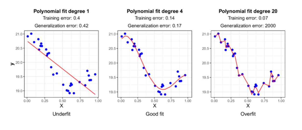Figure 1- Underfitting vs Good fit vs Overfitting.

Figure 1: Underfitting vs Good fit vs Overfitting. Image Source.

On the other hand, overfitting happens when the model tries too hard to follow the training data pattern, leading to poor generalization of unseen data. In other words, it has low bias and high variance. We need to apply regularization techniques to avoid overfitting, which we'll discuss in the next section.

From the bias and variance concept above, the ideal situation would be to have a model with just low enough variance and bias values. However, this is often not feasible due to various reasons, such as noisy data, insufficient data, computation resources, etc. Therefore, the goal is rather to find the sweet spot in the bias-variance trade-off, where the model performs with reasonable accuracy on both the training and test data.

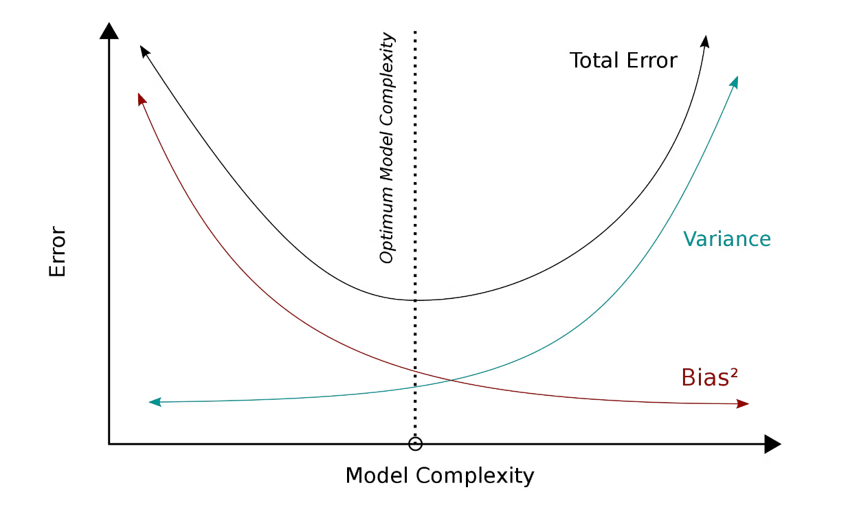Figure 2- Bias and variance trade-off

Figure 2: Bias and variance trade-off. Image Source.

The regularization techniques we'll discuss in the next section aim to reduce the variance of the model, enabling it to generalize well on unseen data.

Different Kinds of Regularization Techniques

There are several regularization techniques available to improve a model's generalization on unseen data. In this section, we'll discuss the most commonly applied ones, including L1 and L2 regularization, Elastic Net, Early Stopping, Dropout, Batch Normalization, and Data Augmentation. Let's start with L1 and L2 regularization.

L1 and L2 Regularization

To understand the concept behind L1 and L2 regularization, let's recap how we optimize the weights of a neural network during the training process.

In each epoch or training step, we need to compute the loss function of our model according to the goal of the task. If it’s a classification, we normally use binary or categorical cross entropy, and if it’s a regression problem, we normally use mean squared error.

Figure 3- Compute the loss function of our model

Figure 3: Compute the loss function of our model

Next, the neural network undergoes an optimization process through a gradient descent algorithm. In this step, first we calculate the partial derivative of the loss function with respect to the weight . Then, we update the weights of our model by subtracting each weight with the multiplication of the derivation result and the learning rate (λ) defined in advance.

Figure 4- Perform gradient descent algorithm

Figure 4: Perform gradient descent algorithm

Both L1 and L2 regularization work by adding a penalty term inside the loss function formula. This term penalizes large weights and pushes them closer towards zero. As you can imagine, if we have a neural network and most of the weights are close or exactly zero, then we'll end up with a much simpler neural network.

One common source of overfitting is a model that's too complex given the training data. By penalizing the weights closer towards zero, we essentially reduce the model's complexity, hence reducing the variance.

The only difference between L1 and L2 regularization is the penalization term added inside the loss function calculation. Let's start with L1 regularization first.

L1 Regularization

In L1 regularization, the additional penalty term inside the loss function would be the multiplication of the sum of all the weights in our model with a penalty parameter α. This penalty parameter needs to be defined in advance and it determines the magnitude of the regularization effect.

If we compute the partial derivative of this additional penalty term with respect to the model weights, we end up with the following equation:

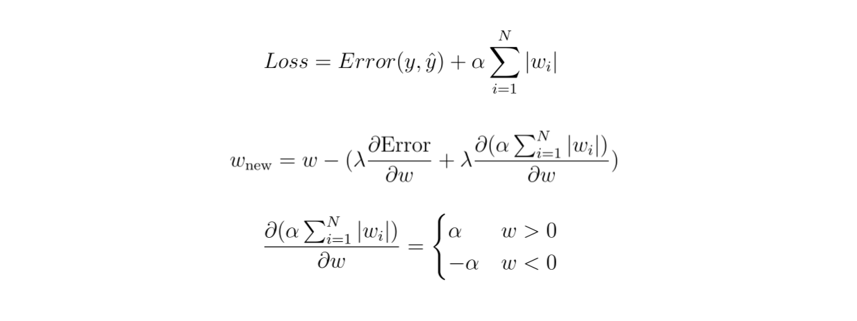Figure 5- Compute the partial derivative of the additional penalty term in L1 regularization

Figure 5: Compute the partial derivative of the additional penalty term in L1 regularization

As you can see, if the weight is positive, the penalty parameter will subtract the weight, making it less positive and closer towards zero. Meanwhile, if the weight is negative, the penalty parameter will add the weight, making it less negative and also closer towards zero.

This regularization method often pushes most weights in a model close to zero, resulting in a less complex model to estimate the data during the training process.

L2 Regularization

The penalty term in L2 regularization is slightly different from L1. L2 regularization implements a squared or L2 norm in the penalty term, as shown in the following equation:

Figure 6- Compute the partial derivative of the additional penalty term in L2 regularization

Figure 6: Compute the partial derivative of the additional penalty term in L2 regularization

If we calculate the partial derivative of the loss function with respect to the weights, we end up with the following equation:

Figure 7- Calculate the partial derivative of the loss function

Figure 7: Calculate the partial derivative of the loss function

As you can see, in L2 regularization, the weight penalty is not solely determined by the sign of the weight itself, but also by its magnitude. As a result, the weights are not pushed towards zero as aggressively as in L1 regularization. However, there's still a chance that the weight becomes zero after this regularization.

Elastic Net

Elastic Net is a method that combines L1 and L2 regularizations into one weighted penalty term added inside the loss function. This means that the sum of the L1 and L2 penalty parameters would add up to one.

Figure 8- Elastic Net

Figure 8: Elastic Net

The main goal of Elastic Net is to enable us to get the best of both L1 and L2 regularizations: it reduces certain features quite effectively as L1 does, but not to the point of aggressively pushing the weights close to zero. On the other hand, it can also reduce the coefficient of not-so-important features effectively, as L2 regularization does.

Let’s now implement L1, L2, and Elastic Net at once. Since Elastic Net is the combination of L1 and L2, we’ll mainly focus on Elastic Net implementation, although you can switch to either L1 and L2 by just commenting out some parts of the code. If you’d like to follow along, all of the code in this article is available in this notebook.

First, let’s import libraries and initialize a 3-layers neural network.

import os
import torch
from torch import nn
from torchvision.datasets import MNIST
from torch.utils.data import DataLoader
from torchvision import transforms
from tqdm import tqdm
from torch.utils.data import Dataset

device = torch.device('cuda' if torch.cuda.is_available() else 'cpu')

class MLP(nn.Module):

     def __init__(self):
         super().__init__()
         self.layers = nn.Sequential(
         nn.Flatten(),
         nn.Linear(28 * 28 * 1, 64),
         nn.ReLU(),
         nn.Linear(64, 32),
         nn.ReLU(),
         nn.Linear(32, 10)
         )

      def forward(self, x):
           return self.layers(x)

      def compute_l1_loss(self, w):
           return torch.abs(w).sum()

      def compute_l2_loss(self, w):
           return torch.square(w).sum()

We implemented the calculation of the penalty term for both L1 and L2 regularization in the model architecture above. Next, let’s define the training procedure for Elastic Net and train the model on MNIST handwritten digits dataset. If you’d like to switch to just L1 or L2, comment out specific parts of the code mentioned in the notebook or in the implementation below:

def train(model, dataset, epochs, lr):

  train_loader = torch.utils.data.DataLoader(dataset, batch_size=10, shuffle=True, num_workers=1)
  loss_function = nn.CrossEntropyLoss()
  optimizer = torch.optim.Adam(model.parameters(), lr=lr)

  for epoch in range(epochs):
    total_loss = 0

    for data in tqdm(train_loader):

        inputs, targets = data
        optimizer.zero_grad()
        outputs = model(inputs.to(device))
        loss = loss_function(outputs, targets.to(device))
        
        l1_weight = 0.4 #Or 1.0 for L1 regularization
        l2_weight = 0.6 #Or 1.0 for L2 regularization

        # Compute L1 and L2 loss component
        # Comment out L1 or L2 depending on regularization you use
        # If you use L1, comment out l2 and vice versa
        parameters = []
        for parameter in model.parameters():
            parameters.append(parameter.view(-1))
        l1 = l1_weight * model.compute_l1_loss(torch.cat(parameters))
        l2 = l2_weight * model.compute_l2_loss(torch.cat(parameters))

        # Add loss component
        # Comment out L1 or L2 depending on regularization you use
        # If you use L1, comment out l2 and vice versa
        loss += l1
        loss += l2
        total_loss += loss.item()

        loss.backward()
        optimizer.step()

    print(f'Epochs: {epoch + 1} | Loss: {total_loss / len(dataset): .3f}')

# train model on MNIST data
EPOCHS = 5
LEARNING_RATE = 1e-4
dataset = MNIST(os.getcwd(), download=True, transform=transforms.ToTensor())
model = MLP().to(device)
train(model, dataset, EPOCHS, LEARNING_RATE)

Early Stopping

Overfitting happens because the model tries too hard to follow the pattern of the training data.** This is particularly common when using an overly complex model and training it on simple data. Therefore, one way to spot and mitigate model overfitting is by observing its performance on validation data during training.

In an ideal scenario, we want the model's error on both training and validation data to decrease in each training iteration. However, if the error on training data continues to decrease while the error on validation data starts to increase, it's an obvious sign that our model overfits the training data.

One way to solve this problem is to train our neural network model for just enough iterations. However, it's almost impossible to know the optimal training iterations for a given dataset in advance. We can, for example, set training iterations as a hyperparameter and then train the model with different iteration values, picking the best model with the best result on validation data. However, this method is inefficient as it requires expensive computational resources, especially when our model is big and complex, and we also have a huge dataset.

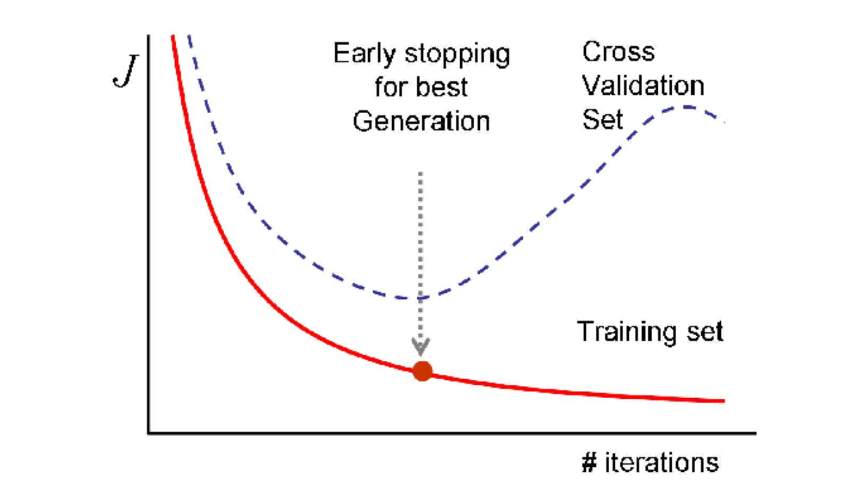Figure 9- Early stopping strategy.

Figure 9: Early stopping strategy. Source.

Early Stopping is a regularization method that solves the problems mentioned above. The concept is simple: we monitor the value of validation loss in each iteration. As soon as the validation loss starts to increase, we stop the training process immediately.**

In practice, it's quite common for a validation loss in an iteration to be higher than the previous one due to randomness during the training process. Therefore, we normally also implement a tolerance value when using Early Stopping. For example, if the tolerance value is set to 2, the method will stop the training process if the validation error doesn't improve in two consecutive iterations.

Let’s implement early stopping with the same model and data that we have implemented in the previous section. We set up the tolerance on validation error to 2, meaning that we’ll stop the training if the validation error doesn’t improve in two consecutive epochs.

def train_with_early_stopping(model, train_dataset, val_dataset, epochs, lr, patience):

  train_loader = torch.utils.data.DataLoader(train_dataset, batch_size=10, shuffle=True, num_workers=1)
  val_loader = torch.utils.data.DataLoader(val_dataset, batch_size=10, shuffle=True, num_workers=1)

  loss_function = nn.CrossEntropyLoss()
  optimizer = torch.optim.Adam(model.parameters(), lr=lr)

  best_loss = 100000
  best_epoch = 0
  for epoch in range(epochs):

        for data in tqdm(train_loader):
        
              inputs, targets = data
              optimizer.zero_grad()
        
              outputs = model(inputs.to(device))
              loss = loss_function(outputs, targets.to(device))
        
              loss.backward()
              optimizer.step()
    
        with torch.no_grad():
              total_loss_val = 0
              for val_data in tqdm(val_loader):
        
                  inputs, targets = val_data
                  outputs = model(inputs.to(device))
        
                  loss = loss_function(outputs, targets.to(device))
                  total_loss_val += loss.item()
    
        avg_loss = total_loss_val / len(val_dataset)
        print(f'Epochs: {epoch + 1} | Val Loss: {avg_loss: .10f}')
    
        if avg_loss < best_loss:
            best_loss = avg_loss
            best_epoch = epoch
            torch.save(model.state_dict(), "best_model.pt")
    
        elif epoch - best_epoch > patience:
            print("Early stopped training at epoch %d" % epoch)
            break  # terminate the training loop

# train the model
PATIENCE = 2
EPOCHS = 1000
LEARNING_RATE = 1e-4
dataset = MNIST(os.getcwd(), download=True, transform=transforms.ToTensor())
train_set, val_set = torch.utils.data.random_split(dataset, [50000, 10000])
model = MLP().to(device)
train_with_early_stopping(model, train_set, val_set, EPOCHS, LEARNING_RATE, PATIENCE)

Dropout

In essence, Dropout is a regularization technique commonly used in neural network architectures by randomly dropping one or several neurons inside a layer during the training process. This means that during training, the weights of dropped neurons won't be updated during the backpropagation process.

To implement Dropout, we first need to define a dropout probability for each layer. As an example, let's say we're setting a 50% dropout probability in a layer. This means that during training, each neuron in that layer has a 50% chance of being dropped. This process occurs independently for each training batch, meaning different subsets of data in the same iteration will most likely have different model architectures due to random neurons being dropped in each layer.

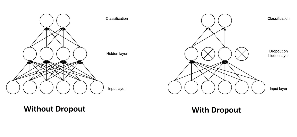Figure 10- Architecture of a neural network before and after dropout.

Figure 10: Architecture of a neural network before and after dropout. Source.

This regularization method is quite destructive, but it's proven to be effective in improving a model's generalization on unseen data. As mentioned in the previous section, one cause of overfitting is an overly complex model. You can imagine that if we randomly drop neurons in each layer, we'll end up with a much simpler model.

Also, if neurons are randomly dropped during training, other neurons need to step in and make necessary weight adjustments to be able to predict the training data correctly. This, in turn, will make the overall model less sensitive to specific weights of neurons in a particular layer, resulting in a model with better generalization capability.

One important thing to note is that we can't drop any neurons in any layers during inference. Therefore, in PyTorch, the activation output of a particular layer during training has been scaled down by 1/1-p, where p is the probability of a neuron in a layer being dropped. We just need to compute an identity function during inference.

In the code implementation below, we’ll create a model with a Dropout layer with 50% probability of dropping neurons. Next, we can train it normally as demonstrated in the previous section.

class MLP_Dropout(nn.Module):

  def __init__(self):
       super().__init__()
       self.layers = nn.Sequential(
         nn.Flatten(),
         nn.Linear(28 * 28 * 1, 64),
         nn.Dropout(p=0.5),
         nn.ReLU(),
         nn.Linear(64, 32),
         nn.Dropout(p=0.5),
         nn.ReLU(),
         nn.Linear(32, 10)
       )

  def forward(self, x):
       return self.layers(x)

model_dropout = MLP_Dropout().to(device)
EPOCHS = 5
train_with_early_stopping(model_dropout, train_set, val_set, EPOCHS, LEARNING_RATE, PATIENCE)

Batch Normalization

Batch Normalization is a technique that normalizes the inputs to a layer by their mean and standard deviation per training batch.

The question then arises: why does Batch Normalization work as a regularization technique?

As you might already know, neural networks are highly sensitive to the setup of the learning algorithm, such as the learning rate, batch size, weight initialization, optimization algorithm, and more. During the training process, the weights of each layer are updated to accurately map input data to the corresponding ground-truth, given the outputs from previous layers.

The issue is that most training data have different distributions, which can cause the learning algorithm to chase a moving target. The weights of one layer can be updated drastically to optimize the mapping of inputs to their label given the activation outputs from the previous layer. As a result, the algorithm needs more iterations to learn. Batch Normalization helps to stabilize and speed up the learning process by normalizing inputs to their mean and standard deviation.

In addition to stabilizing and speeding up the learning process, input normalization also introduces some randomness. This method is typically performed per batch, so inputs have their own mean and standard deviation in each batch. Therefore, the network sees different inputs for each batch, preventing it from memorizing the training data and avoiding overfitting.

Below is an example of how we can implement batch normalization in PyTorch. After implementing the model with batch normalization, then you can train it immediately with the same approach as before.

class MLP_BN(nn.Module):

  def __init__(self):
       super().__init__()
       self.layers = nn.Sequential(
         nn.Flatten(),
         nn.Linear(28 * 28 * 1, 64),
         nn.BatchNorm1d(64),
         nn.ReLU(),
         nn.Linear(64, 32),
         nn.BatchNorm1d(32),
         nn.ReLU(),
         nn.Linear(32, 10)
       )

  def forward(self, x):
       return self.layers(x)

model_bn = MLP_BN().to(device)
EPOCHS = 5
train_with_early_stopping(model_bn, train_set, val_set, EPOCHS, LEARNING_RATE, PATIENCE)

Data Augmentation

Data augmentation is helpful in preventing overfitting for an obvious reason: it helps increase the size of the training data. As mentioned in the previous section, overfitting can occur when training an overly complex model on limited training data. If we somehow manage to increase the training data, the generalization error of our model will decrease.

There are several common data augmentation methods we can implement to increase the data. If we're dealing with images, we can perform image rotation, flipping, scaling, cropping, or shifting. Meanwhile, if we're dealing with text data, we can replace words with their synonyms or use generative AI to generate semantically similar texts.

Below are several examples of image data augmentation with MNIST data:

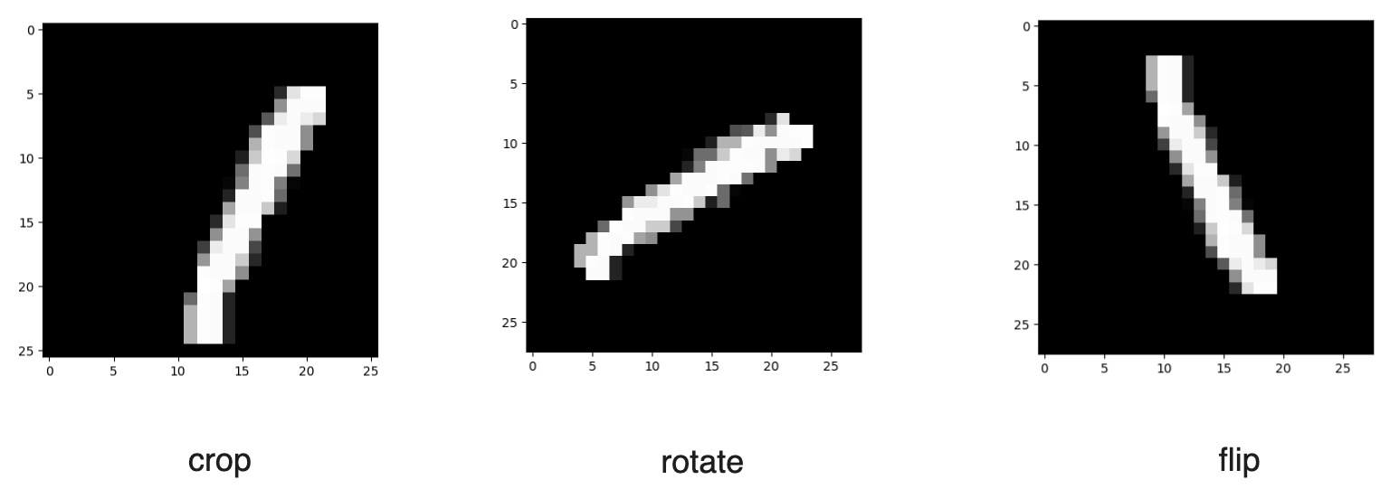Figure 11- Several examples of image augmentation of MNIST handwritten digits dataset.

Figure 11: Several examples of image augmentation of MNIST handwritten digits dataset.

We can perform image data augmentation in PyTorch with the transforms.Compose() method from torchvision library. Inside of this method, you can specify image data augmentation methods that you want to implement.

In the code below, we’ll implement three kinds of image augmentation: crop, flip, and rotation. If you’d like to learn other image augmentation methods, check out this resource from PyTorch.

transform_train = transforms.Compose([
              transforms.ToTensor(),
              transforms.RandomCrop(28, padding=4),
              transforms.RandomVerticalFlip(),
              transforms.RandomRotation(50)])

model = MLP().to(device)
EPOCHS = 5
LEARNING_RATE = 1e-4
dataset = MNIST(os.getcwd(), download=True, transform=transform_train)
train(model, dataset, EPOCHS, LEARNING_RATE)

Conclusion

Overfitting is a condition when a machine learning model tries too hard to follow the pattern of training data, leading to a poor performance on unseen data. Regularization is a technique commonly applied during the training process of a neural network to prevent overfitting.

Several commonly applied regularizations in practice include L1 and L2 regularizations, Elastic Net, Early Stopping, Dropout, Batch Normalization, and Data Augmentation. Although these techniques have different approaches to regularizing a machine learning model, their goal is the same: to reduce the variance and increase the bias of the model. This way, the model can achieve the sweet spot between bias and variance in the bias-variance trade-off.

You can find all the code implemented in this article in this notebook.

Further Resources

Ruben Winastwan

Next: A Beginner's Guide to Understanding Vision Transformers (ViT)

Content

Start Free, Scale Easily

Try the fully-managed vector database built for your GenAI applications.

Try Zilliz Cloud for Free