Learn
AI & Machine Learning

Batch vs. Layer Normalization - Unlocking Efficiency in Neural Networks

Mar 22, 202415 min read

By unraveling the intricacies of layer and batch normalization, we aim to equip neural network beginners with the knowledge to unlock efficiency and enhance model performance.

By Shivek Santosh Maharaj

Read the entire series

Introduction

As deep learning and neural networks grow in complexity and scale, ensuring stable and efficient training becomes increasingly challenging. Efficient training is where batch normalization layers and techniques step in to alleviate some of these challenges. Normalization ensures that the data passed through the network layers remains within manageable ranges. In 2015, a paper titled "Batch Normalization: Accelerating Deep Network Training by Reducing Internal Covariate Shift" from Google presented a batch normalization technique; a year later, a paper titled "Layer Normalization" from the University of Toronto presented a technique on layer normalization.

This article will review these techniques, exploring their distinct functionalities, advantages, applications, and Python syntax. By understanding and comparing layer and batch normalization, we aim to equip beginners in neural networks with the knowledge needed to unlock efficiency and enhance model performance.

Normalization

Understanding Normalization

Normalization is a technique for scaling and shifting input data to ensure it falls within a certain range or distribution. This optimization process not only helps mitigate the effects of varying data distributions but also aids in stabilizing the learning process by ensuring that the inputs to each layer of the neural network are within manageable ranges.

One of the primary challenges that normalization tackles is internal covariate shift. Internal covariate shift refers to the phenomenon of the data going into each neural network layer changing as the network learns. Imagine trying to hit a moving target—it isn't easy to aim accurately. Similarly, when the data keeps changing, it makes it challenging for the network to learn effectively. Normalization helps keep the data more stable, like steadying your aim so the network can learn better and faster.

Normalization alleviates internal covariate shifts by enforcing consistency in the distribution of input data, thereby promoting smoother and more efficient training. By normalizing the inputs, neural networks can maintain a more stable gradient flow, leading to faster convergence and improving the overall efficiency and accuracy of the neural network model.

How does Batch Norm works?

Batch normalization or batch norm is a widely used technique in training, offering a systematic approach to normalizing each layer's inputs across different mini-batches of data. The process involves normalizing the activations of a the mean and variance given layer by subtracting the batch mean and dividing by the batch standard deviation.

The process and formula is as follows:

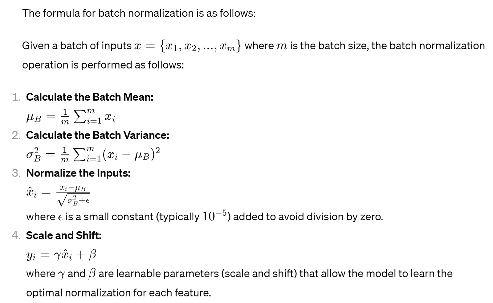
During training, it computes the mean and standard deviation corresponding to the mini-batch by reducing batch and spatial dimensions. By normalizing the inputs within each mini-batch, implement batch normalization norm helps reduce the internal covariate shift, stabilizing the training process and accelerating convergence. This batch normalization layer enables neural networks to learn more efficiently and effectively, especially in deeper architectures where the vanishing or exploding gradient problem may arise.

This normalization process is applied independently to each input tensor feature dimension (channel). The parameters γ and β are learned during training along with the other neural network parameters.

Advantages and Drawbacks of Batch Normalization

The 4 key advantages and potential drawbacks of the batch norm are shown in the table below:


Advantages of Batch Norm	Drawbacks of Batch Norm
Accelerates convergence during training by reducing internal covariate shift.	Dependency on mini batch statistics may limit performance in inference settings where these statistics are unavailable. And it is less suited for sequence models because, in sequence models, we may have sequences of potentially different lengths and smaller batch sizes corresponding to longer sequences.
Stabilizes the training process, allowing for higher learning rates and improved model generalization.	Introduces additional computational overhead during training due to the need to compute batch statistics and normalize activations.
Provides regularization effects, reducing the need for other regularization techniques such as dropout.	Performance may degrade when dealing with small batch sizes or highly variable input distributions.
Mitigates the impact of vanishing or exploding gradients, making it easier to train deep neural networks.	May introduce noise during training, leading to suboptimal performance or convergence issues in certain cases.

Depending on the architecture and design choices, batch normalization can be applied before or after the layer's activation function. Despite its drawbacks, applying batch normalization still remains a valuable tool in the arsenal of neural network practitioners, offering tangible benefits in terms of training efficiency and performance.

What is Layer Normalization?

Layer normalization or layer norm presents an alternative approach to batch normalization. It focuses on normalizing the inputs across features for each layer independently of the batch size. Unlike batch normalization, which operates on mini-batches of data, layer normalization normalizes the activations of each input layer across the entire dataset.

The process involves computing the mean and standard deviation of the activations across features for previous layers within each sample, effectively normalizing the inputs within each layer independently. This ensures that the network remains robust to variations in batch size and facilitates stable training across different datasets and input distributions.

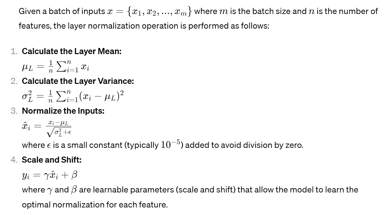
Like batch normalization, this (layer) normalization process is applied independently to each input tensor feature dimension (channel). Layer normalization computes statistics across the feature dimension.

Advantages and Drawbacks of Layer Normalization

The 4 key advantages and potential drawbacks of batch normalization are shown in the table below:


Advantages of Layer Norm	Drawbacks of Layer Norm
Suitable for scenarios with small batch sizes or variable batch sizes, as it normalizes activations independently across features.	May not perform as effectively in scenarios with large batch sizes, where batch normalization might be more suitable.
Robust to changes in input distribution and batch size, making it more stable during training.	Introduces minimal computational overhead during training compared to batch normalization, as it does not require computing batch statistics.
Provides regularization effects like batch normalization, helping to improve model generalization.	May lead to slower convergence compared to batch normalization in certain cases, particularly with large batch sizes and simple network architectures.
Can be applied to recurrent neural networks (RNNs) and transformer-based models, where the input sequence length may vary.	Requires tuning additional hyperparameters such as the normalization scale and shift parameters (gamma and beta).

Layer normalization can be applied before or after the activation function of the layer, depending on the architecture and design choices of previous layer of the hidden layer.

Batch Normalization vs Layer Normalization

Layer and batch norms are powerful tools for stabilizing and accelerating the training process in neural networks. However, they operate on different principles and exhibit distinct characteristics that warrant careful consideration when choosing between them for a particular application. The table below provides a comparative analysis of layer and batch normalization explained, and batch normalization.


Factor	Layer Norm	Batch Norm
Normalization Approach	Normalizes activations across features (per layer).	Normalizes activations across mini-batches (per layer).
Computation	Computes statistics across features.	Computes statistics across mini-batches.
Dependency on Batch Size	No dependency on batch size.	Requires sufficiently large batch sizes for stable training.
Inference Performance****	Suitable for online or real-time inference.	May require additional adjustments for inference due to batch dependencies.
Suitability for Different Model Architectures	- Well-suited for recurrent neural networks (RNNs) and transformer-based models, where input sequence lengths may vary.- Effective in scenarios with small batch sizes or variable batch sizes, as it normalizes activations independently across features.	- Commonly used in feedforward neural networks and convolutional neural networks (CNNs), especially in scenarios with large, consistent batch sizes.- Provides regularization effects and can mitigate the impact of vanishing or exploding gradients, facilitating training of deep networks.
Impact on Model Performance	- Offers stability and robustness across varying batch sizes and input distributions.- May lead to slower convergence compared to batch normalization in certain cases, particularly with large batch sizes and simple network architectures.	- Accelerates convergence during training by reducing internal covariate shift.- Introduces additional computational overhead during training due to the need to compute batch statistics and normalize activations.
Use Cases	- Recurrent neural networks (RNNs)- Transformer-based models- Online or real-time inference scenarios	- Feedforward neural networks- Convolutional neural networks (CNNs)- Scenarios with large, consistent batch sizes

The choice between layer normalization and batch normalization depends on various factors, including the dataset's specific characteristics, the neural network's architecture, and the training environment's computational constraints. While batch normalization excels in stabilizing training dynamics and accelerating convergence, layer normalization offers greater flexibility and robustness, especially in scenarios with small batch sizes or fluctuating data distributions.

Batch and Layer Norm Use Cases

Layer and batch norms find widespread application across various domains, demonstrating their efficacy in enhancing neural network training and performance. Here, we delve into real-world applications and scenarios where these normalization techniques have been effectively implemented:

Image Processing: In computer vision tasks such as object detection and image classification, layer norm and batch norm play crucial roles in stabilizing training dynamics and improving model generalization. These techniques help mitigate the effects of data variability and enhance the robustness of neural network models to variations in lighting conditions, viewpoints, and object scales.
Natural Language Processing (NLP): In NLP tasks such as language modeling, machine translation, and sentiment analysis, normalization is instrumental in addressing the challenges of varying sentence lengths, word distributions, and linguistic nuances. Layer norm and batch norm aid in stabilizing the training process, enabling neural network models to capture long-range dependencies and achieve superior performance on diverse textual datasets.
Reinforcement Learning: In reinforcement learning applications such as game playing and robotics, normalization is crucial in stabilizing the learning process and accelerating policy convergence. Ensuring consistent and stable updates to the policy parameters, layer norm, and batch normalization facilitates more efficient exploration and exploitation strategies, leading to improved learning efficiency and task performance.
Generative Modeling: In generative modeling tasks such as image and text generation, normalization is essential for ensuring the stability and convergence of the training process. Layer norm and batch normalization help mitigate mode collapse and improve the diversity and quality of generated samples, leading to more realistic and coherent outputs.

By exploring these diverse applications and use cases, we gain valuable insights into the versatility and effectiveness of layer and batch normalization across different domains and tasks. In the next section, we'll discuss emerging trends in batch normalization parameters and techniques within neural networks, offering a glimpse into the future of this evolving field. The following section will look at a practical hands-on example of Batch Normalization and Layer Normalization in the Python programming language for Image Recognition.

Batch Norm in Python- Example

We begin by importing all necessary dependencies:

# import all necessary packages
import numpy as np
import matplotlib.pyplot as plt
import tensorflow as tf
from tensorflow.keras.datasets import mnist
from tensorflow.keras.models import Sequential
from tensorflow.keras.layers import Dense, Flatten, BatchNormalization
from tensorflow.keras.optimizers import Adam

We thereafter load the MNIST dataset and preprocess the data:

# load the MNIST dataset
(X_train, y_train), (X_test, y_test) = mnist.load_data()
X_train, X_test = X_train / 255.0, X_test / 255.0

Next, we proceed to define a simple neural network model without batch norm (model_no_bn) as follows:

# define a simple neural network model without batch norm
model_no_bn = Sequential([
    Flatten(input_shape=(28, 28)),
    Dense(128, activation='relu'),
    Dense(64, activation='relu'),
    Dense(10, activation='softmax')
])

Thereafter, we compile and train the model without batch norm:

# compile and train the model without batch norm
model_no_bn.compile(optimizer='adam',
                    loss='sparse_categorical_crossentropy',
                    metrics=['accuracy'])
history_no_bn = model_no_bn.fit(X_train, y_train, epochs=5, validation_data=(X_test, y_test), verbose=2)

We define a simple neural network model with batch norm (model_with_bn):

# define a simple neural network model with batch norm
model_with_bn = Sequential([
    Flatten(input_shape=(28, 28)),
    Dense(128, activation='relu'),
    BatchNormalization(),
    Dense(64, activation='relu'),
    BatchNormalization(),
    Dense(10, activation='softmax')
])

We compile and train the model with batch norm:

# compile and train the model with batch norm
model_with_bn.compile(optimizer='adam',
                      loss='sparse_categorical_crossentropy',
                      metrics=['accuracy'])
history_with_bn = model_with_bn.fit(X_train, y_train, epochs=5, validation_data=(X_test, y_test), verbose=2)

Finally, we visualize the training curves for both models to compare their performance.

# Visualize the training curves
plt.figure(figsize=(10, 5))
plt.subplot(1, 2, 1)
plt.plot(history_no_bn.history['accuracy'], label='Train Accuracy (No BN)')
plt.plot(history_no_bn.history['val_accuracy'], label='Validation Accuracy (No BN)')
plt.xlabel('Epoch')
plt.ylabel('Accuracy')
plt.title('Training Curves without Batch Normalization')
plt.legend()

plt.subplot(1, 2, 2)
plt.plot(history_with_bn.history['accuracy'], label='Train Accuracy (With BN)')
plt.plot(history_with_bn.history['val_accuracy'], label='Validation Accuracy (With BN)')
plt.xlabel('Epoch')
plt.ylabel('Accuracy')
plt.title('Training Curves with Batch Normalization')
plt.legend()

plt.tight_layout()
plt.show()

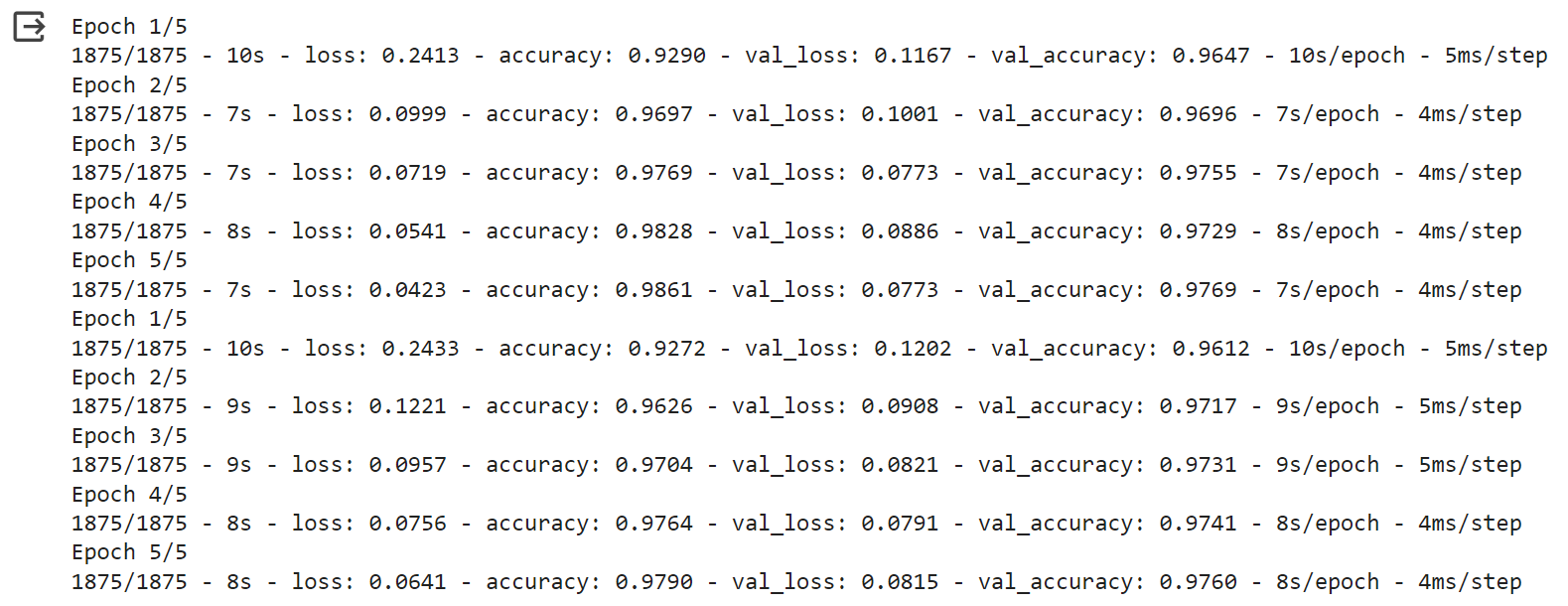
The output to the entire script of code shown above will show as follows (note that your graphs will differ upon every execution):

Deciphering The Output

The training logs show the loss and accuracy values for both training and validation sets for test data at each epoch during the training process.

Interpreting the results:

Loss and Accuracy Trends: Looking at the loss values, we aim for them to decrease over epochs, indicating that the model is improving in its predictions. Correspondingly, we want to see the accuracy values increase, reflecting better performance on both the training and validation datasets.
Faster Convergence: The model with batch normalization seems to converge quicker. "Convergence" refers to the point at which the model's performance stabilizes or reaches a plateau. In this context, it means the model is learning the patterns in the data more rapidly and achieving higher accuracy sooner in the training process.
Learning Rate: While the term "learning rate" usually refers to a hyperparameter in optimization algorithms, here, it can be understood informally as the rate at which the model learns from the training data. A faster convergence often implies a higher effective learning rate, meaning the model updates its parameters more quickly to minimize the loss.

In summary, the model with batch norm demonstrates faster learning and achieves better performance (higher accuracy) in fewer epochs compared to the model without batch norm. This indicates the effectiveness of batch norm in stabilizing and accelerating the training process.

Layer Normalization in Python- Example

We begin by importing all necessary dependencies:

# import all the necessary dependencies
import numpy as np
import matplotlib.pyplot as plt
import tensorflow as tf
from tensorflow.keras.datasets import mnist
from tensorflow.keras.models import Sequential
from tensorflow.keras.layers import Dense, Flatten, LayerNormalization
from tensorflow.keras.optimizers import Adam

We thereafter load the MNIST dataset and preprocess the data:

# load the MNIST dataset
(X_train, y_train), (X_test, y_test) = mnist.load_data()
X_train, X_test = X_train / 255.0, X_test / 255.0

Next, we proceed to define a simple neural network model without layer normalization (model_no_ln) as follows:

# define a simple neural network model without Layer Normalization
model_no_ln = Sequential([
    Flatten(input_shape=(28, 28)),
    Dense(128, activation='relu'),
    Dense(64, activation='relu'),
    Dense(10, activation='softmax')
])

Thereafter, we compile and train the model without layer normalization:

# wompile the model without Layer Normalization
model_no_ln.compile(optimizer='adam',
                    loss='sparse_categorical_crossentropy',
                    metrics=['accuracy'])

# Train the model without Layer Normalization
history_no_ln = model_no_ln.fit(X_train, y_train, epochs=5, validation_data=(X_test, y_test), verbose=2)

We define a simple neural network model with layer normalization (model_with_ln):

# Define a simple neural network model with Layer Normalization
model_with_ln = Sequential([
    Flatten(input_shape=(28, 28)),
    Dense(128, activation='relu'),
    LayerNormalization(),  # Add Layer Normalization layer
    Dense(64, activation='relu'),
    LayerNormalization(),  # Add Layer Normalization layer
    Dense(10, activation='softmax')
])

We compile and train the model with batch norm:

# Compile the model with Layer Normalization
model_with_ln.compile(optimizer='adam',
                      loss='sparse_categorical_crossentropy',
                      metrics=['accuracy'])

# Train the model with Layer Normalization
history_with_ln = model_with_ln.fit(X_train, y_train, epochs=5, validation_data=(X_test, y_test), verbose=2)

Finally, we visualize the training curves for both models to compare their performance.

# Visualize the training curves
plt.figure(figsize=(10, 5))

# Plot training curves without Layer Normalization
plt.subplot(1, 2, 1)
plt.plot(history_no_ln.history['accuracy'], label='Train Accuracy (No LN)', color='blue')
plt.plot(history_no_ln.history['val_accuracy'], label='Validation Accuracy (No LN)', color='orange')
plt.xlabel('Epoch')
plt.ylabel('Accuracy')
plt.title('Training Curves without Layer Normalization')
plt.legend()

# Plot training curves with Layer Normalization
plt.subplot(1, 2, 2)
plt.plot(history_with_ln.history['accuracy'], label='Train Accuracy (With LN)', color='blue')
plt.plot(history_with_ln.history['val_accuracy'], label='Validation Accuracy (With LN)', color='orange')
plt.xlabel('Epoch')
plt.ylabel('Accuracy')
plt.title('Training Curves with Layer Normalization')
plt.legend()

plt.tight_layout()
plt.show()

The output to the entire script of code shown above will show as follows (note that your graphs will differ upon every execution):

Deciphering The Output

The output we observe shows us the training progress of two models, one without Layer Normalization and the other with Layer Normalization, both trained on the MNIST dataset for five epochs.

For the model without Layer Normalization:

Initially, the training accuracy is 92.93%, and the validation accuracy is 96.09%.
After five epochs of training, the training accuracy increases to approximately 98.68%, and the validation accuracy reaches around 97.38%.
Overall, the model without Layer Normalization demonstrates steady improvement in training and validation accuracy over the epochs.

For the model with Layer Normalization:

Similarly, the model starts with a training accuracy of approximately 93.61% and a validation accuracy of around 96.70%.
After five epochs, the training accuracy improves to about 98.70%, while the validation accuracy initially dips to about 96.58% after the third epoch before increasing again to approximately 97.76%.
Despite the temporary dip in validation accuracy after the third epoch, the model with Layer Normalization still achieves a higher validation accuracy than the model without Layer Normalization.

In summary, both models show improvement in training and validation accuracy over the epochs. However, the model with Layer Normalization demonstrates comparable or slightly better performance, even though it experiences a temporary decrease in validation accuracy during training. This highlights the effectiveness of Layer Normalization in stabilizing variance during training and enhancing model performance over time.

Future Directions and Best Practices of Batch and Layer Norm

As the field of neural network training continues to evolve, normalization techniques remain at the forefront of research and innovation. The most prominent emerging trends and future directions in normalization within neural networks are as follows:

Adaptive Normalization: One promising direction is the development of adaptive normalization that dynamically adjusts its parameters during training based on the characteristics of the data and the training dynamics. Adaptive normalization methods aim to enhance the robustness and adaptability of neural network models to varying input distributions and training environments.
Group Normalization: Another area of interest is group normalization, which divides the channels of each layer into groups and computes normalization statistics within each group independently. Group normalization offers an alternative approach to batch and layer normalization, providing increased flexibility and efficiency, especially in scenarios with limited computational resources.
Normalization for Specific Architectures: Techniques tailored to specific neural network architectures, such as recurrent neural networks (RNNs) and transformer-based models, are also gaining attention. Customized normalization layers and strategies can help address these architectures' unique challenges and requirements, further enhancing their performance and efficiency.
Normalization Regularization: Additionally, normalization regularization techniques, which incorporate normalization layers as regularization mechanisms, are being explored to improve model generalization and robustness. By integrating normalization into the regularization framework, practitioners can achieve better control over model complexity and prevent overfitting.

In terms of best practices, beginners in the field of neural networks are encouraged to experiment with different normalization techniques and evaluate their performance on diverse datasets and tasks. Understanding the trade-offs and considerations associated with each normalization method is crucial for making informed decisions in model design and training.

Conclusion

In this blog, we've reviewed the concepts of layer normalization and batch normalization, two techniques in the domain of neural network training in deep learning. By exploring their distinct functionalities, advantages, applications, and practical hands-on examples, we have gained valuable insights into their roles in enhancing model efficiency and performance.

Layer normalization and batch normalization offer complementary approaches to addressing the challenges of internal covariate shift and stabilizing the training process. While batch normalization excels in stabilizing training dynamics and accelerating convergence, layer normalization offers greater flexibility and robustness, especially in scenarios with small batch sizes or fluctuating data distributions.

By understanding their strengths and limitations, practitioners can make informed decisions in model design and training, ultimately leading to more efficient and effective neural network architectures.

In conclusion, layer normalization and batch normalization are indispensable tools in the arsenal of neural network practitioners. They offer powerful mechanisms for stabilizing training dynamics, enhancing model performance, performing natural language processing and computer vision tasks, and unlocking efficiency in neural network architectures. The Zilliz team encourages further exploration and experimentation with these techniques in various machine learning projects, paving the way for continued advancements in the field.

Further resources:

Shivek Santosh Maharaj

Next: Empowering AI and Machine Learning with Vector Databases

Content

Start Free, Scale Easily

Try the fully-managed vector database built for your GenAI applications.

Try Zilliz Cloud for Free

Batch vs. Layer Normalization - Unlocking Efficiency in Neural Networks

Introduction

Understanding Normalization

How does Batch Norm works?

Advantages and Drawbacks of Batch Normalization

What is Layer Normalization?

Advantages and Drawbacks of Layer Normalization

Batch Normalization vs Layer Normalization

Batch and Layer Norm Use Cases

Batch Norm in Python- Example

Deciphering The Output

Layer Normalization in Python- Example

Deciphering The Output

Future Directions and Best Practices of Batch and Layer Norm

Conclusion

Content

Start Free, Scale Easily

Share this article