Learn
AI & Machine Learning

Deep Residual Learning for Image Recognition

Sep 24, 202410 min read

Deep residual learning solves the degradation problem, allowing us to train a neural network while still potentially improving its performance.

By Ruben Winastwan

Read the entire series

The introduction of deep neural networks has opened up many breakthroughs in several areas, such as image classification, image recognition, object detection, and text classification. The high-level intuition behind these breakthroughs is simple: the deeper the network we train, the better its performance will be. Before introducing residual networks, the models with the best performance across different image classification benchmarks tended to have a very deep stack of layers.

The fact that the depth of a neural network seems essential in improving its performance begs the question: Is improving the performance of a deep learning model as simple as stacking more layers?

It turns out that stacking more layers doesn't necessarily lead to better training performance. The root causes of this phenomenon are the vanishing gradient problem and the fact that deeper neural networks are more complicated to optimize. The concept of residual networks was introduced to mitigate these issues and stabilize the training process. In this article, we will discuss residual networks in detail.

Vanishing Gradient and Degradation Problems in Deep Neural Networks

The performance of deep learning models tends to improve as their architecture becomes deeper, as demonstrated in many benchmark datasets. In ImageNet datasets, for example, the models with the best performances have depths ranging from sixteen to thirty layers.

From this observation, it's natural to think that if we want to improve the performance of a neural network, we just need to add more layers to it. The main challenge in proving this hypothesis was the emergence of vanishing gradients during training.

Vanishing gradient is a problem commonly occurring in neural networks with many layers. It refers to a phenomenon where gradients become extremely small as they're back-propagated through numerous layers. As you might imagine, the closer the gradient is to zero, the more difficult it is for a layer to learn in each training iteration. If the gradient is zero, there's nothing for a layer to learn.

Batch normalization is commonly applied during training to solve the vanishing gradient problem. The idea of batch normalization is to normalize the input of each layer such that after it passes through an activation function, the resulting values won't be too large or small. Overall, batch normalization helps the model learn and converge during training.

Thanks to batch normalization, we can train neural networks with a deep stack of layers until they converge and test our assumption that deeper networks always perform better. However, it turns out that adding more layers doesn't always lead to improved performance. Rather, at a particular point, adding more layers will degrade the model's performance and increase training error.

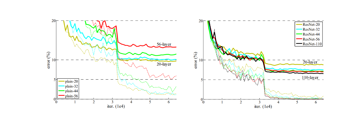Training progress on the CIFAR-10 dataset. Dashed lines denote training error, and bold lines denote testing error. .png

Training error (left) and test error (right) on CIFAR-10 with 20-layer and 56-layer standard networks. Source.

This performance degradation doesn't come from model overfitting but rather from the fact that deeper neural networks are more difficult to optimize. Deep residual learning is a concept introduced to solve this degradation problem, allowing us to train a deep neural network while still potentially improving its performance.

The Concept of Deep Residual Learning

In a nutshell, deep residual learning refers to training deep neural networks using residual connections. A residual connection allows the input of a layer to be directly added to the output of a later layer, creating a shortcut path through the network, as you can see in the following visualization:

Shortcut connection in deep residual learning. .png

Shortcut connection in deep residual learning. Source.

So, how do these residual connections differ from the normal connections between layers in a deep neural network? In a standard deep neural network, each layer's output becomes the input to the next layer, and we can express it mathematically as:

y=fx.png

where y represents the output of a particular layer, and F(x) is the mapping of input to output learned by that layer. With a residual connection, we instead have:

y=fx+x.png

where x is the original input without the mapping process. This means we create a shortcut for input x to add F(x) and x to produce output y.

This simple concept is very helpful in alleviating the vanishing gradients and performance degradation problems. The residual connection makes a deep neural network easier to optimize. If the identity mapping is already optimal, the network only needs to push F(x) to zero, and the shortcut connection will carry the input forward unchanged. Meanwhile, during backpropagation, the gradient can flow directly through the shortcut connection, avoiding potential vanishing in the main path.

Another special feature of this shortcut connection is that it doesn't introduce extra parameters or computational complexity since the element-wise addition of F(x) + x is quite negligible. This makes the concept of residual connection very attractive, and we can also easily compare the performance of a residual neural network with its standard neural network counterpart.

In the next section, we'll compare the performance between residual neural networks and standard neural networks.

Residual Network Performance Comparison

The performance of residual networks has been evaluated on the ImageNet dataset, which is an image classification dataset with 10,000 distinct classes. To compare performance, two standard neural networks were first trained: one with 18 layers and another with 34 layers.

Next, the residual network versions of these two models were also trained on the same dataset and setup. Below is the visualization of the standard network with 34 layers and its residual network version:

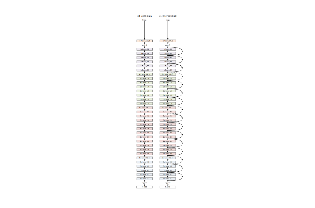Example network architectures of a standard neural network (left) and its residual counterpart (right)..png

Example network architectures of a standard neural network (left) and its residual counterpart (right). Source.

As you can see, the residual network contains several shortcut connections between layers. These shortcut connections don’t introduce extra parameters or computational complexity during model training.

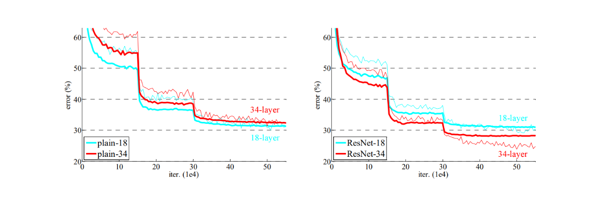
The training results for standard neural networks show that the network with 34 layers has a higher training error than the one with 18 layers throughout the training procedure, as shown in the visualization below. This is an example of performance degradation discussed in the previous section. Networks with more layers are assumed to have higher training errors due to their lower convergence rates and greater difficulty in optimization compared to shallower models.

Training error (left) and test error (right) on CIFAR-10 with 20-layer and 56-layer standard networks..png

Training progress on ImageNet. Thin curves denote training error, and bold curves denote validation error. Source.

Now, if we look at the training results of the residual networks, the network with 34 layers outperforms the one with 18 layers. Not only does the network with 34 layers have a lower training error, but its validation error is also consistently lower, indicating that the model's results are generalizable. This shows that shortcut connections introduced in residual networks are very effective in mitigating the performance degradation problem commonly occurring in deep neural networks.

If we examine the visualization above, we see that the residual network with 18 layers converged faster than the one with 34 layers. This demonstrates that in models with shallower layers, shortcut connections ease the optimization process by providing faster convergence in the early stages. To further evaluate the performance of residual networks, deeper models were built. Specifically, three residual networks were constructed: one with 50 layers, one with 101 layers, and another with 152 layers.

To make shortcut connections more efficient in these deeper networks, their placement was modified. Instead of placing them between a stack of two layers, they are placed between three convolutional layers that mimic a bottleneck design. It’s called a bottleneck design because the three layers have 1x1, 3x3, and 1x1 convolutions. The remarkable aspect is that although the depth of the 152-layer residual model is greater than VGG19, its complexity is lower (11.3 billion FLOPs vs. 19.6 billion FLOPs).

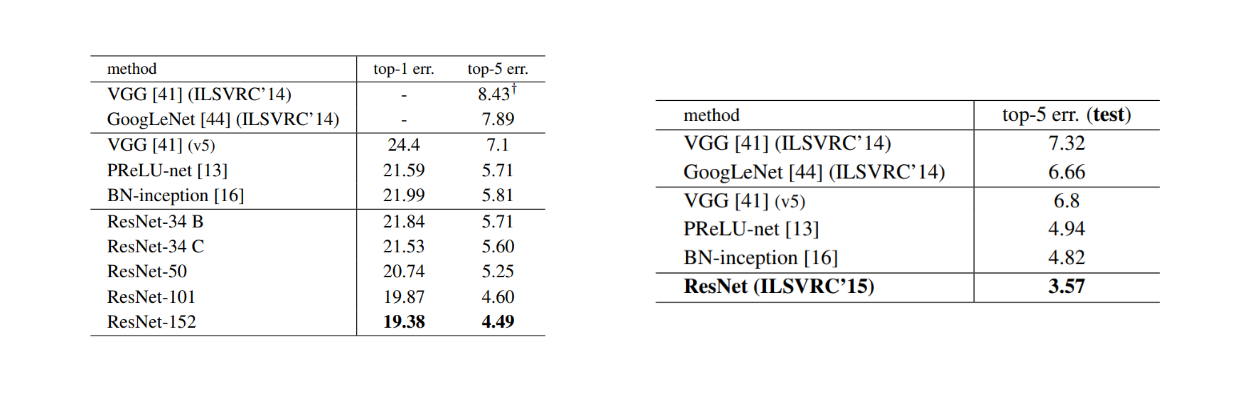Error rates (%) of single-model results (left) and ensembles (right)..png

Error rates (%) of single-model results (left) and ensembles (right). Source.

As you can see, we can still enjoy performance gains as model depth increases due to these shortcut connections. The error on validation ImageNet data shows that the deepest model with 152 layers is superior to any other residual network variants and state-of-the-art models like VGG, GoogLeNet, and PReLU-net.

This residual method demonstrates consistent performance not only on the ImageNet dataset but also across different datasets and machine learning use cases. In the visualization below, residual networks outperform their standard counterparts throughout the training process by recording lower training and validation errors on the CIFAR dataset.

Training progress on ImageNet. Thin curves denote training error, and bold curves denote validation error..png

Training progress on the CIFAR-10 dataset. Dashed lines denote training error, and bold lines denote testing error. Source.

In object detection tasks, residual networks also outperform state-of-the-art models like VGG on both PASCAL and MS COCO datasets. As shown in the table below, the mean average precision (mAP) of residual networks is higher than that of VGG.

Object detection mAP (%) on the PASCAL VOC (left) and COCO dataset (right)..png

Object detection mAP (%) on the PASCAL VOC (left) and COCO dataset (right). Source.

The consistent performance and flexibility of residual networks across different datasets have led to their adaptation not only in computer vision tasks but also in natural language tasks, where the residual concept is found within famous architectures such as Transformers.

Residual Networks Implementation

In this section, we’ll see how residual networks can be used for an image classification use case. We’ll load a pre-trained residual network and then use it to predict an image's class.

We can use torchvision library from PyTorch to load pre-trained residual networks with the following code:

import torch
from torchvision import models, transforms
from PIL import Image
import requests
from io import BytesIO


# Download and load the pre-trained ResNet model
model = models.resnet50(pretrained=True)
model.eval()

In the above code, we load a pre-trained residual network with 50 layers. However, you can also load networks with more layers, such as the ones with 101 and 152 layers or the smaller ones with 34 and 18 layers.

Next, since we want to predict an image into one of the 10,000 classes available on the ImageNet dataset, we also need to load the name of these 10,000 classes as a mapping from our model’s prediction to the actual name of the predicted class.

# Download ImageNet class labels
LABELS_URL = "<https://raw.githubusercontent.com/pytorch/hub/master/imagenet_classes.txt>"
response = requests.get(LABELS_URL)
labels = [line.strip() for line in response.text.splitlines()]
print(labels)


"""
Output:
['tench', 'goldfish', 'great white shark', 'tiger shark', 'hammerhead', 'electric ray', 'stingray', ....]
"""

Before we can predict an image with residual networks, we need to transform it. This step includes resizing our image into the same dimension as the training data and then normalizing it according to some mean and standard deviation gathered from the training data.

The ImageNet training data has an image size of 256 x 256. Meanwhile, the mean and standard deviation are [0.485, 0.456, 0.406] and [0.229, 0.224, 0.225], respectively, where each element in the list refers to one channel. We can also do all of these transformations at once with the `torchvision` library.

transform = transforms.Compose([
    transforms.Resize(256),
    transforms.CenterCrop(224),
    transforms.ToTensor(),
    transforms.Normalize(mean=[0.485, 0.456, 0.406], std=[0.229, 0.224, 0.225]),
])

We’ll try to predict an image of a tiger cat, as shown in the visualization below.

image_url = "<https://upload.wikimedia.org/wikipedia/commons/thumb/3/3a/Cat03.jpg/1200px-Cat03.jpg>"

Test image. .png

Test image.

The final step before we can predict an image is to create a predict function. This function takes our image as an input. Then, we transform the image with the code we’ve written above, call the model to obtain the prediction, and map the prediction into one of the classes available on ImageNet.

def predict(image_url):

    response = requests.get(image_url)
    img = Image.open(BytesIO(response.content))
    
    img_t = transform(img)
    batch_t = torch.unsqueeze(img_t, 0)
    
    with torch.no_grad():
        output = model(batch_t)
    
    _, predicted_idx = torch.max(output, 1)
    predicted_label = labels[predicted_idx.item()]
    
    return predicted_label

Now, let’s predict the image by calling the function.

prediction = predict(image_url)
print(f"The image is predicted to be: {prediction}")
"""
Output:
The image is predicted to be: tiger cat
"""

Conclusion

Introducing deep residual learning has solved problems related to vanishing gradients and performance degradation commonly occurring in deep neural networks. By introducing shortcut connections that allow the input of a layer to be directly added to the output of a later layer, we can train much deeper networks with performance gains. These shortcut connections make deep networks easier to optimize and train efficiently without adding significant computational complexity or extra parameters.

Residual networks have also proven versatile, being implemented in many machine learning use cases, such as image classification, object detection, and object localization. The concept of residual connections has not only been successful in computer vision tasks but has also been adapted to other areas of deep learning, such as natural language processing, where it has been incorporated into architectures like Transformers.

Further Resources

Ruben Winastwan

Next: Decoding Transformer Models: A Study of Their Architecture and Underlying Principles