RoBERTa: An Optimized Method for Pretraining Self-supervised NLP Systems
Pre-trained language models have achieved striking success in natural language processing (NLP), leading to a paradigm shift from supervised learning to pre-training followed by fine-tuning. The goal of language modeling is to predict the next token in a sequence, given a history of unannotated texts, which are large amounts of raw text data that have not been labeled with specific information. BERT (Bidirectional Encoder Representations from Transformers) sets new standards for this concept by enabling bidirectional language understanding as it looks at the whole sentence, not just one word at a time. It considers the words before and after to understand their meaning better.
However, the primary issue found with BERT was its undertraining, which limited its performance on NLP tasks. This limitation led the researchers to explore improved training methodologies in subsequent models, like RoBERTa.
RoBERTa (A Robustly Optimized BERT Pretraining Approach) is an improved version of BERT designed to address its limitations. RoBERTa introduced several key improvements that enhance its performance across various NLP problems.
This article will discuss methodologies and technologies used in RoBERTa's development, including its training approach, the results it has achieved, and the potential future research opportunities it opens up.
A Quick Intro to BERT (Bidirectional Encoder Representations from Transformers)
To understand RoBERTa, it's essential to understand its predecessor, BERT, and the challenges it faced. BERT introduced the concept of bidirectional transformers, enabling deep learning models to understand the context in a previously unattainable way.
But, to really understand how BERT works, we need to break it down. So, let's take a closer look at its architecture and how it was trained.
BERT’s architecture and pre-training process
BERT's architecture is based on transformers, introduced by Devlin et al. in 2018. It uses a multi-layer bidirectional (left-to-right and right-to-left) encoder to weigh the importance of different words in a sentence.
 BERT Architecture
Figure 1: BERT Architecture
A word starts with its embedding representation from the embedding layer; an embedding is a dense vector (numerical representation) of a word or token in a high-dimensional space. The embedding layer is the first layer in a neural network that converts input words into these dense vectors. Every layer performs multi-headed attention computations on the previous layer's word representation to generate a new intermediate representation. All of these intermediate representations are of equal size. In the figure above, E1 is the embedding representation, T1 is the final output, and Trm is the token's intermediate representation.
BERT's pre-training process includes two main tasks:
Masked Language Modeling (MLM)
Next-Sentence Prediction (NSP)
Language modeling predicts the next word given a sequence of words. In the MLM task, though, instead of predicting every next token, a percentage of input tokens is masked randomly, and only those masked tokens are predicted. The NSP task, on the other hand, is a binary classification task that predicts whether two given sentences follow each other in the original text. This approach helps the model understand the relationships between sentences.
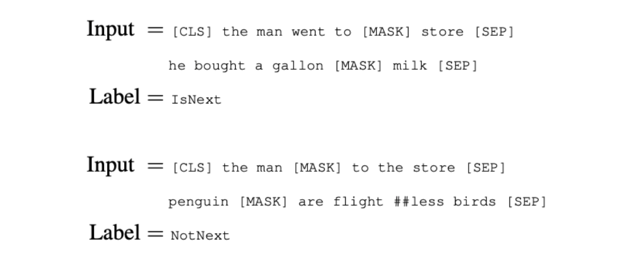 Next Sentence Prediction
Figure 2: Next Sentence Prediction
BERT's pre-training process had limitations that kept it from reaching its full potential. One of the primary issues was using a static masking pattern in the MLM task. In BERT, once a word was masked during training, the same words were masked across all iterations. This static approach limited the model to diverse masking scenarios, reducing its generalization ability. Furthermore, the training data size and duration were also limited.
These limitations led to inconsistencies in BERT's performance on domain-specific tasks, such as legal or medical text analysis, and complex language understanding scenarios, like sentiment analysis or multi-step reasoning. Addressing these shortcomings requires further research and development.
The Emergence of RoBERTa
The primary motivation behind RoBERTa's development was to address the challenges observed in BERT's pre-training process. However, RoBERTa maintains the same core architecture as Bert Large, which consists of 24 layers, 1024 hidden units, and 16 attention heads, totaling 355 million parameters.
The challenges RoBERTa aimed to address were:
Static masking pattern: BERT's static masking led to limited training scenarios, causing overfitting. Overfitting occurs when a model performs very well for training data but performs poorly with test data (new data). RoBERTa introduced dynamic masking, generating new masks for each epoch and improving its ability to handle new data.
Insufficient training data: BERT's training was based on a dataset of approximately 16 GB of text, which is insufficient to capture the full diversity of language. RoBERTa scaled up the training data, using over 160 GB of text from various sources.
Short training duration: The original BERT model was trained for a relatively short duration, but RoBERTa extended the training duration significantly, running for more epochs and iterations.
Small batch sizes and conservative learning rates: BERT's pretraining used relatively small batch sizes and conservative learning rates, which was a safe but limiting approach. On the other hand, RoBERTa experimented with larger batch sizes and more aggressive learning rates, which led to better model performance.
What is RoBERTa and How Does It Work?
RoBERTa (A Robustly Optimized BERT Pretraining Approach) is an improved version of BERT designed to address its limitations for improved performance. It introduced modifications to the BERT's training process that improve its performance on natural language processing tasks.
These modifications include:
Dynamic masking
Removal of the NSP
Larger Training Data and Extended Duration
Increasing batch sizes
Byte text encoding
Dynamic masking
From BERT’s architecture, we remember that during pre-training, BERT performed Masked Language Modeling (MLM) by trying to predict a certain percentage of masked tokens. These chosen masked tokens were the same (static) in each iteration.
RoBERTa addressed this issue by implementing a slightly better approach called dynamic masking. This approach changes the masking scheme every time a sequence is passed to BERT during training. This change made the training data more varied, allowing the model to learn a wider range of language patterns. As a result, RoBERTa developed a deeper understanding of context, which improved performance on downstream tasks.
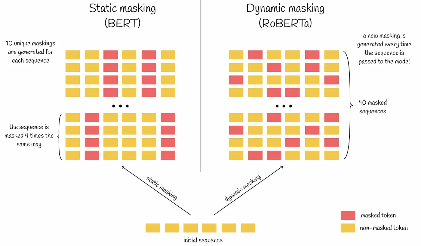 Static masking vs. dynamic masking
Figure 3: Static masking vs. dynamic masking
The researchers who developed RoBERT also reimplemented the static masking approach by duplicating the training data 10 times. This duplication allowed each sequence to be masked in ten different ways over the 40 training epochs. Thus, each training sequence was seen with the same mask four times during training. The performance was similar when comparing the reimplementation of static masking to the original BERT model. However, dynamic masking shows slightly better performance than static masking.
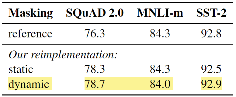 Comparison between static and dynamic masking
Figure 4: Comparison between static and dynamic masking
Removal of the next sentence prediction (NSP)
Another key modification in RoBERTa was the removal of the NSP task. In NSP, the model was given pairs of sentences and had to predict whether the second sentence followed the first in the original text. However, RoBERTa's development found that the NSP task contributed minimally to the model's performance on downstream tasks.
RoBERTa uses a FULL-SENTENCES approach (packing sequences from multiple documents). Each input to the model is packed with full sentences sampled contiguously from one or more documents up to the maximum sequence length of 512 tokens. This allows the model to learn long-range dependencies more effectively.
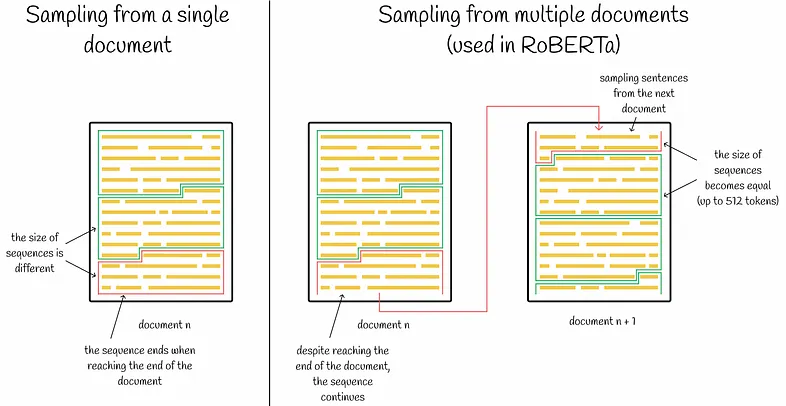 BERT with and without NSP
Figure 5: BERT with and without NSP
Additionally, the researchers looked at four different ways to format input data for a language model. They compared two main formats: the original SEGMENT-PAIR and SENTENCE-PAIR. Both formats use NSP, but the SENTENCE-PAIR format uses single sentences instead of pairs. The researchers found that using single sentences made the model perform worse on tasks because it struggled to understand connections between words far apart in the text.
Next, they tested the model by training it without the NSP method and using blocks of text from a document called DOC-SENTENCES. In most cases, they found it did better than the original BERT, and not using the NSP loss didn't hurt the model's performance.
The text from a single document (DOC-SENTENCES) method was slightly better than that from multiple documents (FULL-SENTENCES). However, since DOC-SENTENCES led to different batch sizes during training, they decided to use FULL-SENTENCES for the rest of their experiments. This choice made it easier to compare their results with those of other related studies.
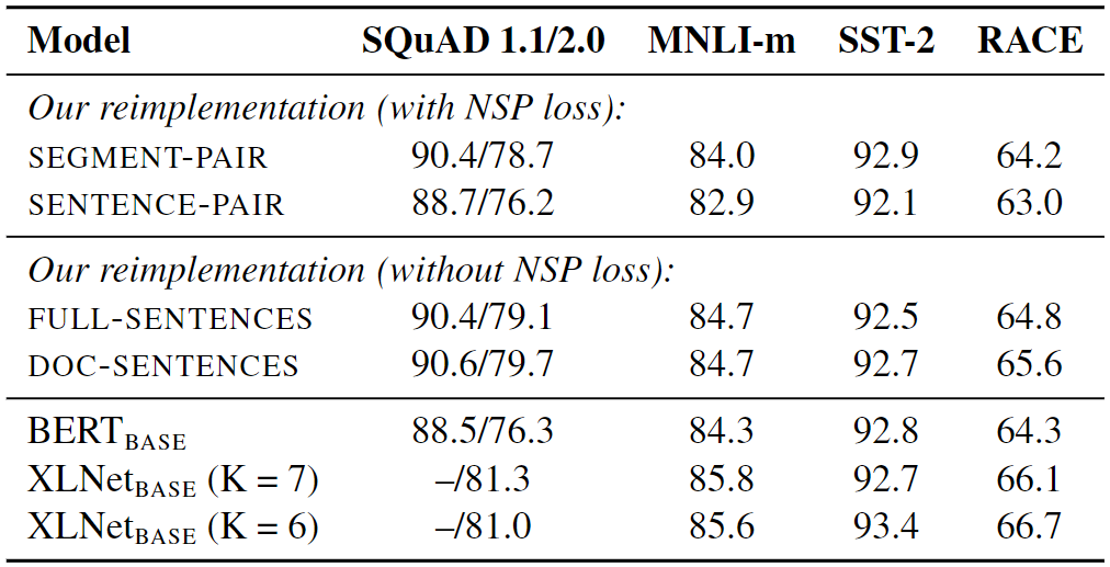 Results for base models pre-trained over BOOK CORPUS and WIKIPEDIA
Figure 6: Results for base models pre-trained over BOOK CORPUS and WIKIPEDIA
Larger training data and extended duration
Perhaps the most straightforward optimization, but no less important, is simply training on more data for a longer time. BERT was trained on a dataset of approximately 16 GB of text, and RoBERTa used over 160 GB of text.
RoBERTa Datasets:
BOOK-CORPUS and WIKIPEDIA: Same as BERT.
CC-NEWS: RoBERTa introduces a new dataset called CC-NEWS, a large-scale news dataset featuring contemporary language and a wide range of topics, styles, and perspectives.
Additional Datasets: RoBERTa combines the above datasets with three other private datasets described in the paper, improving performance on downstream tasks.
Using larger training data, extending the training duration, and running for more epochs and iterations, RoBERTa shows a large improvement of 4-6% on downstream tasks compared to the originally reported BERT results (Devlin et al. in 2018).
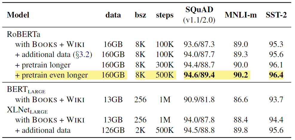 Results for RoBERTa over the BERT
Figure 7: Results for RoBERTa over the BERT
Increasing batch sizes
Past work in neural machine translation has shown that training with very large mini-batches can improve perplexity for masked language modeling. This approach improves end-task performance when the learning rate is increased appropriately (Ott et al., 2018). Perplexity is a metric used to measure the performance of language models. It quantifies the uncertainty (probability distribution) a model has when predicting the next word in a sequence. For instance, the lower the perplexity and the more accurate the predictions.
Based on this concept, RoBERTa uses much larger mini-batches during training. Whereas BERT used a batch size of 256 sequences for a million steps, RoBERTa increased this to 8k sequences for 31k steps with a learning rate value of 1e-3. However, optimal performance was seen with 2k sequences for 125k steps.
 Comparison of Perplexity and End-Task Performance of BERT vs. RoBERTa
Figure 8: Comparison of Perplexity and End-Task Performance of BERT vs. RoBERTa
Byte text encoding
RoBERTa also introduced an alternative method for handling out-of-vocabulary (OOV) words by employing byte-level Byte Pair Encoding (BPE). BERT used a character-level Byte-Pair Encoding (BPE) vocabulary of 30K units. RoBERTa expands this to a byte-level BPE vocabulary of 50K subword units without additional input preprocessing or tokenization. Compared to BERT, this method allowed RoBERTa to encode almost any word or subword without using the unknown token.
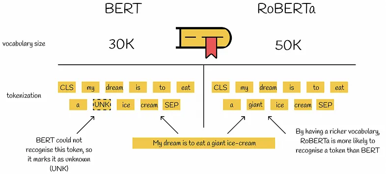 Byte text encoding
Figure 9: Byte text encoding
Experiment Results
After modifying BERT(Devlin et al. 2019), RoBERTa was tested on NLP benchmarks. We will discuss its performance on three benchmarks: GLUE, SQuAD, and RACE.
GLUE (General Language Understanding Evaluation): A collection of 9 datasets for NLU (natural language understanding) tasks.
SQuAD (Stanford Question Answering Dataset): A dataset designed for training and evaluating question-answering systems. It consists of real questions posed by humans on a set of Wikipedia articles, where the answer to each question is a specific span of text within the corresponding article.
RACE (Reading Comprehension from Examinations): A large-scale reading comprehension dataset was collected from English exams.
Testing results on the GLUE dataset
RoBERTa was tested using two fine-tuning settings. In the first setting (single-task), RoBERTa was separately fine-tuned for 10 epochs for each GLUE task, using only the training data for the corresponding task. It achieved state-of-the-art results on all nine GLUE tasks, outperforming both BERT and XLNet. In the second setting (ensembles), RoBERTa scored 88.5 on the GLUE leaderboard, matching the previous state-of-the-art set by XLNet. RoBERTa set new state-of-the-art results on 4 of 9 GLUE tasks: MNLI, QNLI, RTE, and STS-B.
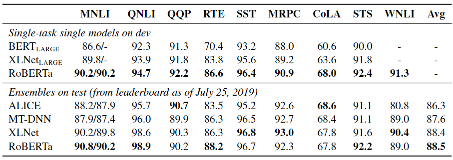 Results on GLUE
Figure 10: Results on GLUE
SQuAD
RoBERTa was fine-tuned using the SQuAD training data. On SQuAD v1.1, RoBERTa matches the state-of-the-art set by XLNet. On SQuAD v2.0, RoBERTa achieved an F1 score of 89.4, setting a new state-of-the-art for single models without data augmentation. This is particularly impressive given that RoBERTa doesn't use any SQuAD-specific techniques and is only fine-tuned on SQuAD data.
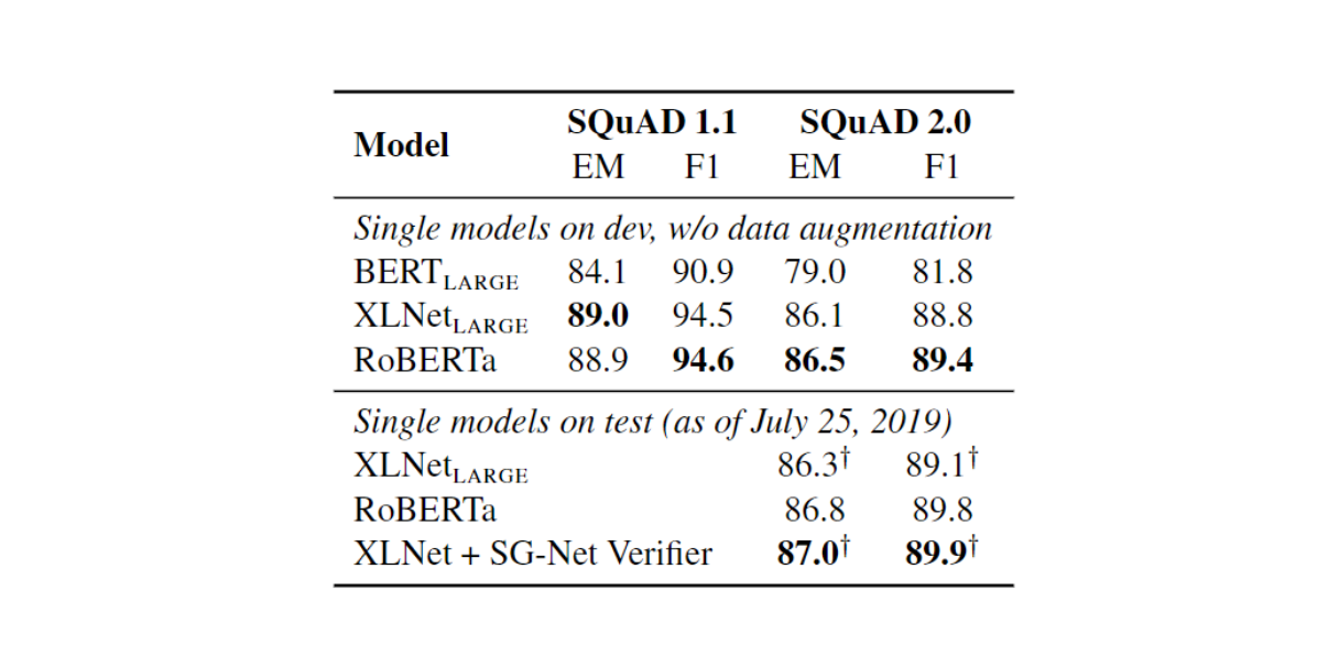 Results on SQuAD
Figure 11: Results on SQuAD
Testing results on the RACE dataset
RACE is a challenging reading comprehension benchmark that requires models to answer multiple-choice questions based on passages from English exams. This benchmark is particularly difficult because it requires models to understand complex passages and infer the correct answers based on context. RoBERTa achieved an accuracy of 83.2% on the RACE benchmark and set new state-of-the-art standards.
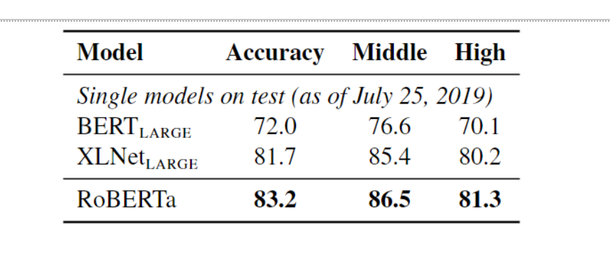 Results on the RACE test set
Figure 12: Results on the RACE test set
Fine-Tuning RoBERTa for Sentiment Analysis
Beyond its performance on standard benchmarks, RoBERTa has also proven highly effective for fine-tuning specific tasks, such as sentiment analysis. Fine-tuning is taking a pre-trained model and adapting it to a specific task by training it on a smaller, task-specific dataset. The source code used in this article is from Hugging Face.
Importing and preparing the dataset
We will use the dataset available at the Kaggle Competition and only refer to the first csv file from the data dump: train.tsv.
Importing Python libraries:
!pip install transformers==3.0.2
Import the libraries and modules needed to run our script at this step.
# Importing the libraries needed
import pandas as pd
import numpy as np
import torch
import transformers
import json
from tqdm import tqdm
from torch.utils.data import Dataset, DataLoader
from transformers import RobertaModel, RobertaTokenizer
import logging
logging.basicConfig(level=logging.ERROR)
# Setting up the device for GPU usage
from torch import cuda
device = 'cuda' if cuda.is_available() else 'cpu'
Preparing the dataset
First, load the dataset and read it using the Pandas package.
train = pd.read_csv('train.tsv', delimiter='\t')
new_df = train[['Phrase', 'Sentiment']]
Let's define some variables:
MAX_LEN: The maximum length of the input text (256).
TRAIN_BATCH_SIZE and VALID_BATCH_SIZE: The batch sizes for training and validation (8 and 4, respectively).
LEARNING_RATE: The learning rate for the model (1e-05).
Tokenizer: A RobertaTokenizer instance is used to preprocess the text data.
The SentimentData class implements a custom dataset class, taking a data frame, tokenizer, and maximum length as inputs. It preprocesses the text data, returning a dictionary containing input IDs, attention masks, token type IDs, and target sentiment labels.
The DataLoader class creates data loaders for the training and testing sets, iterating over the data in batches during training and validation.
# Defining some key variables that will be used later on in the training
MAX_LEN = 256
TRAIN_BATCH_SIZE = 8
VALID_BATCH_SIZE = 4
LEARNING_RATE = 1e-05
tokenizer = RobertaTokenizer.from_pretrained('roberta-base', truncation=True, do_lower_case=True)
class SentimentData(Dataset):
    def __init__(self, dataframe, tokenizer, max_len):
        self.tokenizer = tokenizer
        self.data = dataframe
        self.text = dataframe.Phrase
        self.targets = self.data.Sentiment
        self.max_len = max_len

    def __len__(self):
        return len(self.text)

    def __getitem__(self, index):
        text = str(self.text[index])
        text = " ".join(text.split())

        inputs = self.tokenizer.encode_plus(
            text,
            None,
            add_special_tokens=True,
            max_length=self.max_len,
            pad_to_max_length=True,
            return_token_type_ids=True
        )
        ids = inputs['input_ids']
        mask = inputs['attention_mask']
        token_type_ids = inputs["token_type_ids"]

        return {
            'ids': torch.tensor(ids, dtype=torch.long),
            'mask': torch.tensor(mask, dtype=torch.long),
            'token_type_ids': torch.tensor(token_type_ids, dtype=torch.long),
            'targets': torch.tensor(self.targets[index], dtype=torch.float)
        }
train_size = 0.8
train_data=new_df.sample(frac=train_size,random_state=200)
test_data=new_df.drop(train_data.index).reset_index(drop=True)
train_data = train_data.reset_index(drop=True)

print("FULL Dataset: {}".format(new_df.shape))
print("TRAIN Dataset: {}".format(train_data.shape))
print("TEST Dataset: {}".format(test_data.shape))

training_set = SentimentData(train_data, tokenizer, MAX_LEN)
testing_set = SentimentData(test_data, tokenizer, MAX_LEN)
train_params = {'batch_size': TRAIN_BATCH_SIZE,
                'shuffle': True,
                'num_workers': 0
                }

test_params = {'batch_size': VALID_BATCH_SIZE,
                'shuffle': True,
                'num_workers': 0
                }

training_loader = DataLoader(training_set, **train_params)
testing_loader = DataLoader(testing_set, **test_params)
Creating the neural network for fine-tuning
We will be creating a neural network with RobertaClass.
This network will have the Roberta Language model, followed by a dropout, and finally, a linear layer to obtain the final outputs.
The data will be fed to the Roberta Language model as defined in the dataset.
The final layer output will be compared to the sentiment category to determine the accuracy of the model's prediction.
We will initiate an instance of the network called Model. This instance will be used for training.
class RobertaClass(torch.nn.Module):
    def __init__(self):
        super(RobertaClass, self).__init__()
        self.l1 = RobertaModel.from_pretrained("roberta-base")
        self.pre_classifier = torch.nn.Linear(768, 768)
        self.dropout = torch.nn.Dropout(0.3)
        self.classifier = torch.nn.Linear(768, 5)

    def forward(self, input_ids, attention_mask, token_type_ids):
        output_1 = self.l1(input_ids=input_ids, attention_mask=attention_mask, token_type_ids=token_type_ids)
        hidden_state = output_1[0]
        pooler = hidden_state[:, 0]
        pooler = self.pre_classifier(pooler)
        pooler = torch.nn.ReLU()(pooler)
        pooler = self.dropout(pooler)
        output = self.classifier(pooler)
        return output
model = RobertaClass()
model.to(device)
Fine-tuning the model
After all the effort of loading and preparing the dataset and creating the model. This is probably the easier step in the process.
Here, we define a training function that trains the model on a specified number of epochs on the above training dataset. An epoch defines how often the complete data will be passed through the network.
# Creating the loss function and optimizer
loss_function = torch.nn.CrossEntropyLoss()
optimizer = torch.optim.Adam(params =  model.parameters(), lr=LEARNING_RATE)
def calcuate_accuracy(preds, targets):
    n_correct = (preds==targets).sum().item()
    return n_correct
# Defining the training function on the 80% of the dataset for tuning the distilbert model
def train(epoch):
    tr_loss = 0
    n_correct = 0
    nb_tr_steps = 0
    nb_tr_examples = 0
    model.train()
    for _,data in tqdm(enumerate(training_loader, 0)):
        ids = data['ids'].to(device, dtype = torch.long)
        mask = data['mask'].to(device, dtype = torch.long)
        token_type_ids = data['token_type_ids'].to(device, dtype = torch.long)
        targets = data['targets'].to(device, dtype = torch.long)

        outputs = model(ids, mask, token_type_ids)
        loss = loss_function(outputs, targets)
        tr_loss += loss.item()
        big_val, big_idx = torch.max(outputs.data, dim=1)
        n_correct += calcuate_accuracy(big_idx, targets)

        nb_tr_steps += 1
        nb_tr_examples+=targets.size(0)

        if _%5000==0:
            loss_step = tr_loss/nb_tr_steps
            accu_step = (n_correct*100)/nb_tr_examples
            print(f"Training Loss per 5000 steps: {loss_step}")
            print(f"Training Accuracy per 5000 steps: {accu_step}")

        optimizer.zero_grad()
        loss.backward()
        # # When using GPU
        optimizer.step()

    print(f'The Total Accuracy for Epoch {epoch}: {(n_correct*100)/nb_tr_examples}')
    epoch_loss = tr_loss/nb_tr_steps
    epoch_accu = (n_correct*100)/nb_tr_examples
    print(f"Training Loss Epoch: {epoch_loss}")
    print(f"Training Accuracy Epoch: {epoch_accu}")
    return
EPOCHS = 1
for epoch in range(EPOCHS):
    train(epoch)
Output:
 Figure 13- Details of the model training
Validating the model performance
During the validation stage, we pass the unseen data (the testing dataset) to the model. This step determines how well the model performs on the unseen data, which is 20% of train.tsv, which was separated during the dataset creation stage.
The validation stage checks the model's generalization ability to new, unseen data. The model's weights have not been updated. Only the final output is compared to the actual value, which is then used to calculate the model's accuracy.
The valid function implements the validation stage, taking the model and testing loader as inputs. It sets the model to evaluation mode, initializes variables to track correct and incorrect predictions, and iterates over the testing loader. For each batch, it calculates the loss and accuracy, printing the validation loss and accuracy at every 5000 steps and the end of the epoch. Finally, it returns the epoch accuracy.
def valid(model, testing_loader):
    model.eval()
    n_correct = 0; n_wrong = 0; total = 0; tr_loss=0; nb_tr_steps=0; nb_tr_examples=0
    with torch.no_grad():
        for _, data in tqdm(enumerate(testing_loader, 0)):
            ids = data['ids'].to(device, dtype = torch.long)
            mask = data['mask'].to(device, dtype = torch.long)
            token_type_ids = data['token_type_ids'].to(device, dtype=torch.long)
            targets = data['targets'].to(device, dtype = torch.long)
            outputs = model(ids, mask, token_type_ids).squeeze()
            loss = loss_function(outputs, targets)
            tr_loss += loss.item()
            big_val, big_idx = torch.max(outputs.data, dim=1)
            n_correct += calcuate_accuracy(big_idx, targets)

            nb_tr_steps += 1
            nb_tr_examples+=targets.size(0)

            if _%5000==0:
                loss_step = tr_loss/nb_tr_steps
                accu_step = (n_correct*100)/nb_tr_examples
                print(f"Validation Loss per 100 steps: {loss_step}")
                print(f"Validation Accuracy per 100 steps: {accu_step}")
    epoch_loss = tr_loss/nb_tr_steps
    epoch_accu = (n_correct*100)/nb_tr_examples
    print(f"Validation Loss Epoch: {epoch_loss}")
    print(f"Validation Accuracy Epoch: {epoch_accu}")

    return epoch_accu

acc = valid(model, testing_loader)
print("Accuracy on test data = %0.2f%%" % acc)
Output:
 Figure 14- Details of the model validation
As you can see, the model predicts the correct category of a given sample with a 69.47% accuracy, which can be further improved by training more.
Future Research Opportunities
RoBERTa’s success has opened new doors for research in NLP and model optimization. Here are some potential research opportunities:
Scaling datasets
Larger datasets and longer training times improved RoBERTa. Future research could investigate dynamic dataset scaling, where models are trained on progressively larger datasets over time. This approach could help us understand how the model learns from new data and if it can keep improving as its data scales.
Multi-task fine-tuning
RoBERTa's performance could be further improved by exploring advanced multi-task fine-tuning procedures. Right now, it's good at lots of things without being trained on multiple tasks at once. However, researchers may investigate how integrating multiple tasks during the fine-tuning phase could improve performance across different benchmarks.
Exploration of pre-training objectives
Removing the NSP objective and using a dynamic masking approach over static masking in RoBERTa raise concerns about whether there are even better ways to teach language models. Future research can explore different pre-training methods that affect how well RoBERTa understands and completes tasks.
Conclusion
The RoBERTa paper makes several important contributions to the field of NLP. The authors find that dynamically changing the masking pattern in the training data, training on longer sequences, and removing the NSP task can improve performance on downstream tasks.
Additionally, using a larger batch size and training dataset also contributes to this improvement. RoBERTa achieves state-of-the-art results on GLUE, RACE, and SQuAD without multi-task fine-tuning for GLUE or additional data for SQuAD.
Furthermore, the debate between RoBERTa and BERT is not just about which model is better. It’s about understanding the trade-offs between computational resources, model performance, and the ethical implications of deploying these models. RoBERTa’s advancements over BERT show that the field of NLP is far from static and opens the door to a path to more advanced and complex language processing capabilities.
Further Resources
Keep Reading

The AWS Outage Was a Wake-Up Call for Vector Database Cross-Region Disaster Recovery
Zilliz Cloud Had the Answer Before the Crisis. Zilliz Cloud is the world's first vector database with native cross-region disaster recovery.

Migrating from S3 Vectors to Zilliz Cloud: Unlocking the Power of Tiered Storage
Learn how Zilliz Cloud bridges cost and performance with tiered storage and enterprise-grade features, and how to migrate data from AWS S3 Vectors to Zilliz Cloud.

Zilliz Named "Highest Performer" and "Easiest to Use" in G2's Summer 2025 Grid® Report for Vector Databases
Zilliz shines in G2's Summer 2025 Grid® Report as both "Highest Performer" and "Easiest to Use," solving the performance-usability dilemma.
