Efficient Memory Management for Large Language Model Serving with PagedAttention
PagedAttention and vLLM solve important challenges in serving LLMs, particularly the high costs and inefficiencies in GPU memory usage when using it for inference.
Read the entire series
- OpenAI's ChatGPT
- Unlocking the Secrets of GPT-4.0 and Large Language Models
- Top LLMs of 2024: Only the Worthy
- Large Language Models and Search
- Introduction to the Falcon 180B Large Language Model (LLM)
- OpenAI Whisper: Transforming Speech-to-Text with Advanced AI
- Exploring OpenAI CLIP: The Future of Multi-Modal AI Learning
- What are Private LLMs? Running Large Language Models Privately - privateGPT and Beyond
- LLM-Eval: A Streamlined Approach to Evaluating LLM Conversations
- Mastering Cohere's Reranker for Enhanced AI Performance
- Efficient Memory Management for Large Language Model Serving with PagedAttention
- LoRA Explained: Low-Rank Adaptation for Fine-Tuning LLMs
- Knowledge Distillation: Transferring Knowledge from Large, Computationally Expensive LLMs to Smaller Ones Without Sacrificing Validity
- RouteLLM: An Open-Source Framework for Navigating Cost-Quality Trade-Offs in LLM Deployment
- Prover-Verifier Games Improve Legibility of LLM Outputs
- Be like a Goldfish, Don't Memorize! Mitigating Memorization in Generative LLMs
- Unlocking the Power of Many-Shot In-Context Learning in LLMs
- Spotting LLMs With Binoculars: Zero-Shot Detection of Machine-Generated Text
- Teaching LLMs to Rank Better: The Power of Fine-Grained Relevance Scoring
- Everything You Need to Know About LLM Guardrails
- Chain-of-Retrieval Augmented Generation
- Chain of Agents (COA): Large Language Models Collaborating on Long-Context Tasks
Large Language Models (LLMs) are powerful and versatile AI systems capable of solving numerous problems across various sectors. Their development is very fast-paced, with new models being released frequently. Generally, newer LLMs exhibit better performance in addressing a variety of tasks. Some of these models, such as Mistral, Llama, OPT, and Qwen, are open-sourced, allowing us to utilize them on our internal data and for commercial purposes.
However, one of the major challenges in implementing these open-source LLMs arises during the serving stage. Hosting LLMs is notably expensive in terms of operational costs, as multiple GPUs are required. Therefore, it is crucial to implement a solution that efficiently manages memory during this stage. One potential solution is the implementation of an algorithm called PagedAttention, which we will discuss in this article.
The Problems with LLM Inference
At their core, LLMs consist of a massive stack of Transformer decoders. As you may know, Transformer decoder-based architecture works by generating text sequentially. This means that the longer the generated text, the more GPU memory is required to run these LLMs.
For example, if you look at GPT-4 pricing, a model with an 8k context window is cheaper than one with a 128k context window. This price difference simply reflects the cost of outputting more text. Additionally, we must consider the model size. As shown in the image below, when hosting an LLM with 13B parameters on an NVIDIA A100, 65% of the GPU memory would be allocated to store the model's weights, 30% for the Key-Value (KV) cache (or context windows), and the remainder for the model's activation.
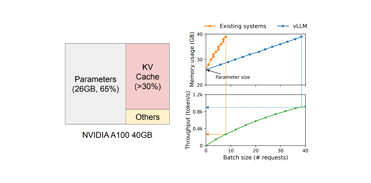 Figure: GPU memory allocation when serving an LLM with 13B parameters
It's well-known that running an open-source LLM as a hosted service is very expensive and requires multiple GPUs. Therefore, increasing throughput and reducing cost per request is crucial. So how do we achieve this? From the GPU memory consumption perspective, the model's weights are fixed, and we can't do much about that. Meanwhile, activation occupies only a small fraction of the GPU memory. Thus, optimizing memory management within the KV cache should be the main focus for improving throughput.
However, the main challenge of optimizing the KV cache lies in the nature of LLM output generation. As mentioned earlier, Transformer-decoders generate text output sequentially, potentially leading to heavy underutilization of the GPU during the inference process.
An obvious improvement in GPU memory utilization and throughput is the ability to perform batched requests. However, implementing batched requests in an LLM is difficult for two reasons:
Requests may arrive at different times. A naive batching strategy would either make earlier requests wait for later ones or delay incoming requests until earlier ones finish, leading to queueing delays.
The requests might have varying input and output lengths, as shown in the token distribution of the ShareGPT and Alpaca datasets below. The straightforward solution is to implement padding so that each request has a similar length, but this wastes memory.
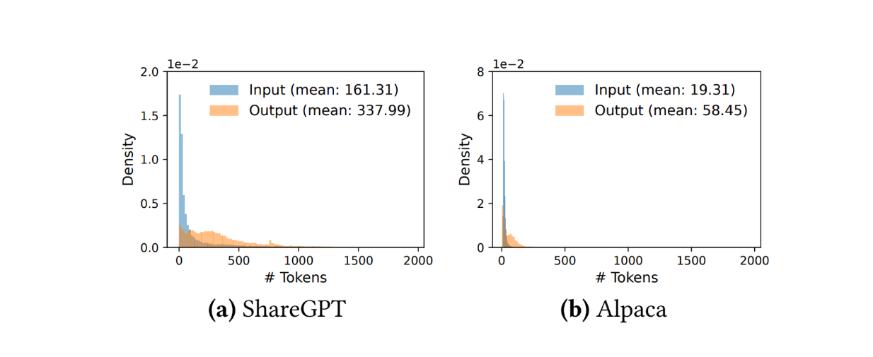 Figure: Input-output length distributions of ShareGPT and Alpaca datasets
Methods called cellular batching and iteration-level scheduling have been implemented to address these issues. These methods operate at the iteration level instead of the request level. Instead of waiting for the entire batch, a new request can be processed as soon as an iteration has finished.
Although cellular batching and iteration-level scheduling solve the problem related to GPU memory utilization, the number of requests that can be processed in a batch is still constrained by GPU memory capacity. Fortunately, the nature of how the KV cache works leaves room for possible improvements. In its implementation, the KV cache has unique characteristics in consuming GPU memory: it can dynamically grow and shrink over time as the model generates new tokens, and its length is not known in advance.
 Figure: KV cache memory management in common methods
When using an LLM for inference, we typically need to set a maximum number of generated tokens (e.g., 1000, 2048, etc.). The GPU then allocates a contiguous chunk of memory according to this maximum length. This approach potentially wastes memory, as in most scenarios, the generated tokens are much shorter than the maximum length.
As shown below, profiling results indicate that only 20.4% - 38.4% of the KV cache memory is actually used to store tokens.
 Figure: The average percentage of memory wastes in different LLM serving systems
A second potential improvement relates to memory sharing of the KV cache. LLMs can generate multiple versions of outputs for a single prompt per request. It would be beneficial if the KV cache could be shared among multiple versions of outputs to optimize GPU memory consumption. However, memory sharing is currently not possible because the KV cache per request is stored in separate contiguous spaces.
To address these issues, a method called PagedAttention has been introduced, which we'll discuss in detail in the next section.
How PagedAttention and vLLM Works
PagedAttention is a method that enables the storage of continuous key-value pairs in non-contiguous memory space. Let's consider a request with the prompt: "Four score and seven years ago, our fathers brought forth."
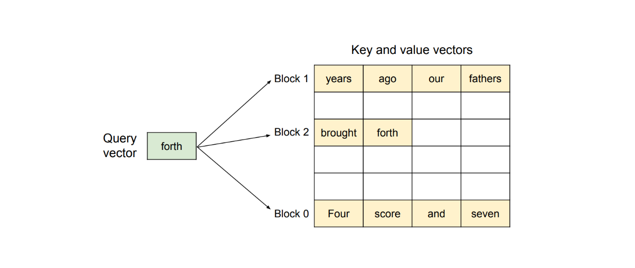 Figure: PagedAttention algorithm visualization
The PagedAttention method first partitions this request's KV cache into KV blocks. Each KV block contains the KV vectors of a fixed number of tokens.
As visualized above, PagedAttention partitions our prompt into three non-contiguous KV blocks within the physical memory. During computation, the method identifies and fetches each KV block separately to compute the attention of the next possible token with respect to previous tokens.
This PagedAttention method is implemented under the hood inside an LLM serving engine called vLLM, which is also introduced in the paper.
vLLM contains a centralized scheduler to coordinate the execution of distributed GPU workers and a KV cache manager. The main goal of the KV cache manager is to effectively manage the KV cache in a paged fashion. The implementation of this manager is inspired by operating systems (OS), which partition memory into fixed-sized pages and create a mapping of user programs from logical pages to physical pages.
The benefit of this implementation is that contiguous logical pages can correspond to non-contiguous physical pages. This means we don't need to reserve physical memory in advance as traditional KV cache systems do, thereby eliminating memory waste in GPU utilization.
To map the logical pages to physical pages in each request, the KV cache manager utilizes a block table. A block table keeps a record of the location of each KV block in both logical and physical pages, as well as the number of filled and unfilled positions, as visualized below.
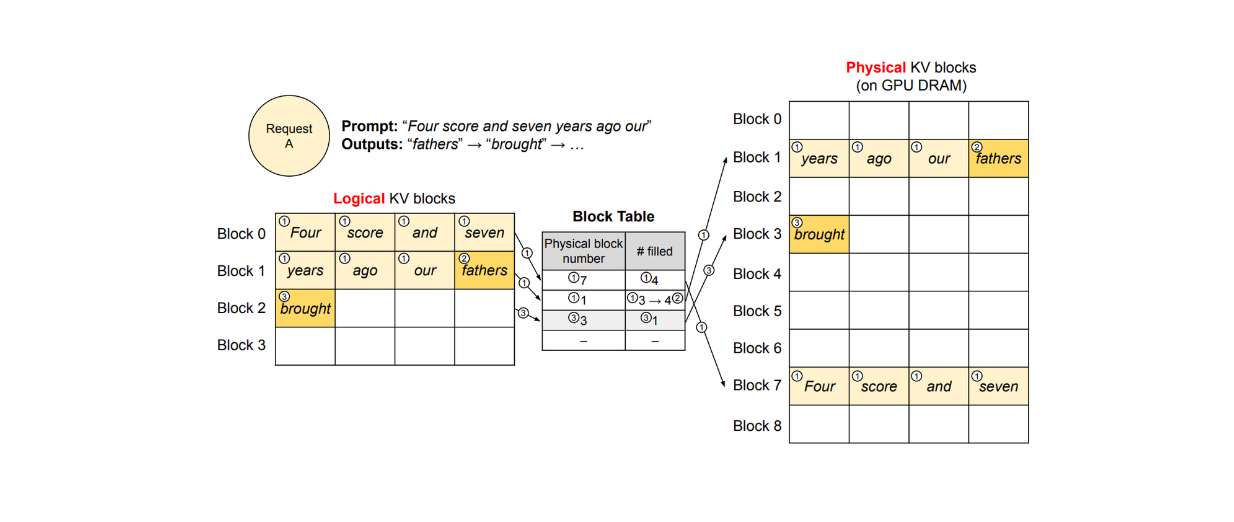 vLLM decoding workflow of a single sample per request
Decoding Process with PagedAttention and vLLM
In this subsection, we'll examine how PagedAttention and vLLM work in detail for a single request.
Let's say we make a request with a prompt containing 7 tokens, as you can see in the visualization above, where each KV block can store 4 tokens. In this case, vLLM initially allocates 2 logical blocks to store the KV of our prompt, which we'll call block 0 and block 1. vLLM then maps these logical blocks to 2 physical KV blocks (blocks 1 and 7 in the visualization) and records this mapping in the block table.
During the text generation process, since the last slot of logical block 1 is still available, vLLM stores the newly generated token there. Next, the #filled record in the block table is updated, as shown in step 2 of the visualization.
At the second iteration, when all slots in the logical blocks are filled, vLLM allocates a new logical block. It then stores the new token there, allocates a new physical block (block 3 in the visualization), and records this mapping in the block table. Once a request is completed, its corresponding KV blocks can be freed for use by other requests.
This method allows more requests to fit into the GPU memory and ensures that no GPU memory is wasted. In the case of multiple requests, the logical blocks of different requests will be mapped to different physical blocks, as illustrated in the visualization below.
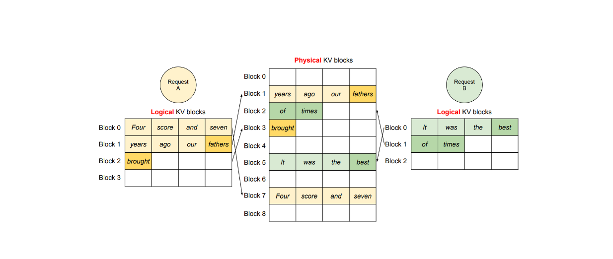 Figure: vLLM decoding workflow of two different requests
Parallel Sampling
vLLM and PagedAttention can also handle many other advanced decoding scenarios, such as parallel sampling.
When we want an LLM to output multiple versions of an output, vLLM provides an efficient solution that allows one KV cache for a prompt to be shared to generate multiple outputs. The main idea is that one physical block can be mapped to multiple logical blocks, and therefore, vLLM introduces a variable called reference count.
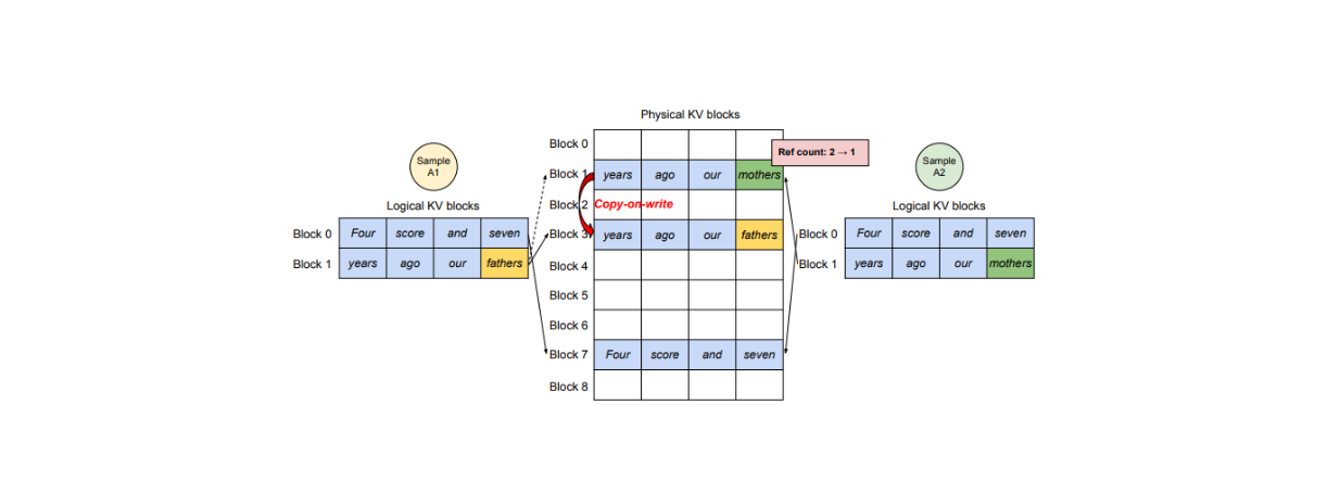 vLLM decoding workflow of parallel sampling
The reference count represents how many logical blocks are mapped to a specific physical block. If we want the LLM to generate two versions of output, A, and B, then the reference count for a particular physical block would be 2.
During the text generation phase, if sample A needs to write into its last slot of a logical block, vLLM checks the reference count of its corresponding physical block. If the reference count is greater than 1, vLLM creates a copy of that block into a new physical block and reduces the reference count to 1. Subsequently, if sample B needs to write into its last logical block, the new KV cache can be stored inside the original physical block since the reference count is now 1.
The concept of parallel sampling is also beneficial in scenarios where we want to create a system prompt. A system prompt is a set of instructions and tasks that we provide to the LLM as input, and this system prompt might not change for several requests. In this case, vLLM can reserve physical blocks to store the KV cache of the system prompt and then perform several text generations similar to the steps explained above.
In its parallel sampling implementation, vLLM also supports the sharing of not only the prompt blocks but also other blocks across different samples. This is particularly useful in beam search scenarios, where we want to retain the top k candidates in every iteration during the text generation process.
Scheduling and Preemption
When hosting an LLM for inference, we may encounter situations where traffic requests exceed the system's capacity. In such cases, vLLM implements first-come-first-served (FCFS) scheduling to ensure that the earliest request is processed first.
However, this scheduling implementation can potentially lead to problems. For example, we might encounter a situation where vLLM runs out of physical blocks in the GPU to store the newly created KV cache of a certain request. In this case, the solution is to discard some physical blocks to free up space. To accomplish this, vLLM implements a method where all physical blocks belonging to a sequence are discarded at once.
This approach raises an important question: what if we need the discarded blocks in the future? Is there a way to recover them? vLLM implements two approaches to address this problem:
Swapping: vLLM's architecture includes a CPU allocator. When blocks are discarded from GPU memory, vLLM copies them into this CPU memory for future use.
Recomputation: If needed, vLLM can simply recompute the KV cache of the requested sequence.
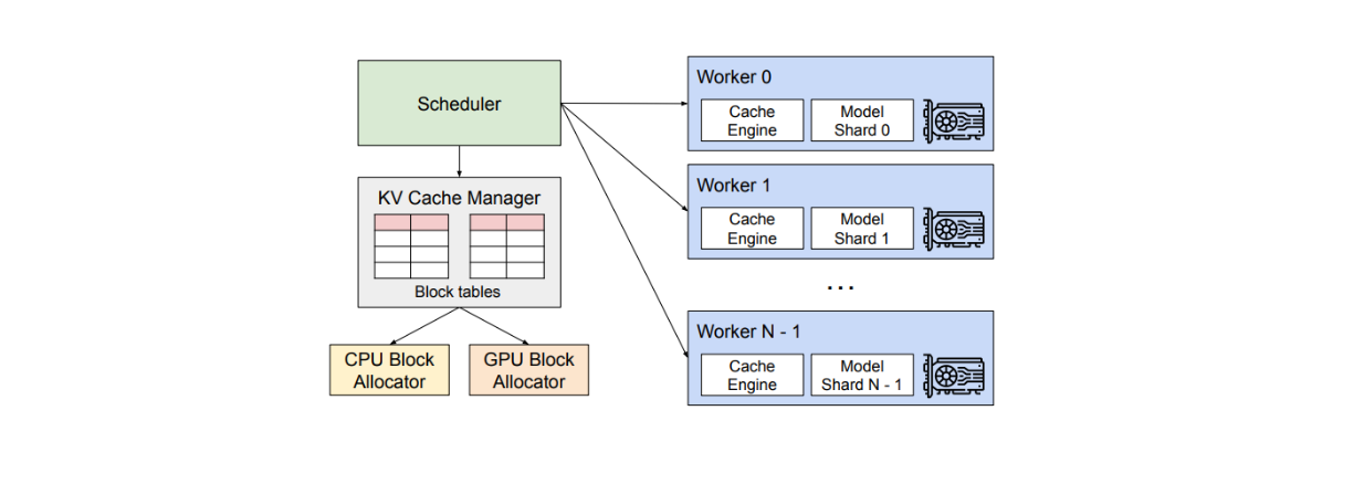 vLLM system overview
vLLMs Performance on Benchmark Datasets
To evaluate the performance of vLLM against other LLM serving methods, several tests with different LLMs and datasets were conducted.
Two different LLM types were used during the test: OPT models with 13B, 66B, and 175B parameters and LLAMA with 13B parameters. The datasets used were the ShareGPT dataset, which contains user-shared conversations with ChatGPT, and the Alpaca dataset, which contains data generated by GPT-3.5-instruct.
The methods compared with vLLM in the paper are FasterTransformer and self-implemented Orca with different setups:
Orca (Oracle): assumes that the system knows the number of tokens generated in a request.
Orca (Pow2): assumes that the system over-reserves the space memory by at most 2x the actual generated tokens.
Orca (Max): assumes that the system reserves the space memory by the maximum length of generated tokens defined in advance (e.g., 2048 tokens).
In basic sampling with the OPT 175B model (i.e., outputting one sample per request), the visualization below shows that vLLM can sustain 1.7x - 2.7x higher throughput than Orca (Oracle) and 2.7x - 8x higher than Orca (Max) on the ShareGPT dataset. On the same dataset, vLLM is far superior to FasterTransformer, sustaining 22x more throughput.
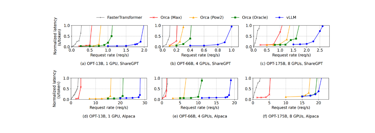 Figure: Single sample generation with OPT models on the ShareGPT and Alpaca dataset
A similar phenomenon occurs with the Alpaca dataset. However, the advantage of using vLLM on this dataset is not as apparent as with the ShareGPT dataset. This is because the OPT 175B model requires large GPU memory to store the KV cache, but the average sequence length of this dataset is much shorter than ShareGPT.
For parallel sampling and beam search, vLLM offers greater performance benefits as more sequences are needed to sample. For example, the improvements of using vLLM increase on the Alpaca dataset from 1.3x with basic sampling to 2.3x with beam search (width of 6), as shown in the visualization below:
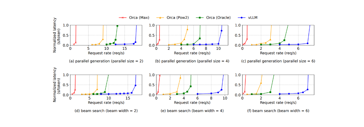 Figure: Parallel generation and beam search with OPT model on the Alpaca dataset
vLLM performed better than other methods in terms of GPU memory saving during parallel sampling and beam search. It results in 6.1%—9.8% more memory saving during parallel sampling and up to 55.2% memory saving during beam search.
 Figure: Average memory saving from sharing KV blocks with OPT 13B on the Alpaca dataset
There is a parameter that can be tweaked when implementing vLLM: the block size, and it's important to choose an appropriate value for block size. If it's too small, vLLM might not be able to fully utilize the GPU's parallelism. Meanwhile, if it's too large, internal fragmentation increases. From observations on the ShareGPT and Alpaca datasets, it can be concluded that a block size of 16 provides a good estimate to fully utilize the powerful performance of vLLM. Therefore, the default block size of vLLM is set to 16.
vLLM Implementation
In this section, we will briefly implement a simple use case with vLLM. Specifically, we will perform an offline inference based on an input prompt. The easiest way to get started with vLLM is by installing it via pip install.
pip install vllm
Now we can install the necessary libraries and then define the list of input prompts, as you can see below:
from vllm import LLM, SamplingParams

prompts = "Hello, my name is"

sampling_params = SamplingParams(temperature=0.8, top_p=0.95)
Inside of SamplingParams class above, you can define the sampling parameters used to generate text outputs, such as the temperature of the LLM, top p, top k, number of output sequences, etc. You can see the complete list of parameters inside this class that you can modify in this documentation.
Next, let’s initialize the LLM and then generate the output with the given prompt. We’re going to implement the Microsoft Phi model with 1.5B parameters. You can check the list of supported models by vLLM in this documentation.
llm = LLM(model="facebook/opt-125m")

outputs = llm.generate(prompts, sampling_params)

# Print the output

prompt = output.prompt

generated_text = output.outputs[0].text

print(f"Prompt: {prompt!r}, Generated text: {generated_text!r}")
vLLM Integration with Milvus
Now that you know the basic implementation of vLLM, let’s build a simple Retrieval Augmented Generation (RAG) by using vLLM and Milvus. Milvus is a vector database that enables you to store millions of vectors and perform a vector search on them in seconds.
The easiest way to get started with Milvus is by installing Milvus Lite, and you can install it via pip install like so:
!pip install -U pymilvus

!pip install pymilvus[model]
Now let’s create a collection and then insert data into it. In the below example, we’re going to insert three text data into our Milvus database by first transforming our text data into vector embeddings. Next, we store the vector embeddings alongside the metadata like subject and original text into Milvus.
from pymilvus import MilvusClient

from pymilvus import model

client = MilvusClient("milvus_demo.db")

# Create collection

if client.has_collection(collection_name="rag_vllm"):

    client.drop_collection(collection_name="rag_vllm")

client.create_collection(

    collection_name="rag_vllm",

    dimension=768,  # The vectors we will use in this demo has 768 dimensions

)

# Define embedding model

embedding_fn = model.DefaultEmbeddingFunction()

# Text data to search from.

docs = [

    "Artificial intelligence was founded as an academic discipline in 1956.",

    "Alan Turing was the first person to conduct substantial research in AI.",

    "Born in Maida Vale, London, Turing was raised in southern England.",

]

# Transform text data into embeddings

vectors = embedding_fn.encode_documents(docs)

data = [

    {"id": i, "vector": vectors[i], "text": docs[i], "subject": "history"}

    for i in range(len(vectors))

]

# Insert embeddings into Milvus

res = client.insert(collection_name="rag_vllm", data=data)
At this stage, we have our data inside Milvus. Next, we can fetch the most relevant data in our Milvus database according to our query.
Let’s say that now we have a question like “What's Alan Turing achievement?”, we can get the most relevant text by performing a vector search. But before that, we need to transform our query into an embedding using the same embedding model that we used to transform text in the database.
SAMPLE_QUESTION = "What's Alan Turing achievement?"

query_vectors = embedding_fn.encode_queries([SAMPLE_QUESTION])

res = client.search(

    collection_name="demo_collection",

    data=query_vectors,

    limit=1,

    output_fields=["text"],

)

context = res[0][0]["entity"]["text"]
And now we have the most relevant data according to our query. In a RAG application, we use the most relevant data as a context that will be used by an LLM to generate contextualized answers to our query. By providing an LLM with relevant context, we reduce the hallucination risk from the LLM.
Now let’s create a complete prompt that we’ll send to our LLM. In a RAG application, the prompt consists of a combination of a high-level task or instruction, our original query, as well as the context fetched from the vector search implemented above.
SYSTEM_PROMPT = f"""Answer the question using the provided Context.

Be clear, concise, relevant.

Context: {context}

User's question: {SAMPLE_QUESTION}

"""

prompts = [SYSTEM_PROMPT]
And finally, we can perform RAG with Microsoft Phi 1.5B model that we also used in the implementation in the previous section.
from vllm import LLM, SamplingParams

sampling_params = SamplingParams(temperature=0.8, top_p=0.95)

llm = LLM(model="microsoft/phi-1_5")

outputs = llm.generate(prompts, sampling_params)

# Print the output

prompt = output.prompt

generated_text = output.outputs[0].text

print(f"Prompt: {prompt!r}, Generated text: {generated_text!r}")

"""

Output:

Question: "What's Alan Turing achievement?"

Generated text: "Answer: Alan Turing's achievement in AI is his pioneering work in developing the concept"

"""
And that’s it! Now you have successfully performed a simple RAG with Milvus, vLLM, and Microsoft Phi. If you’d like to know more in detail about Milvus integration with vLLM, check out the documentation page.
Conclusion
In this article, we’ve discussed a paper that introduced us to PagedAttention and vLLM. PagedAttention and vLLM solve important challenges in serving LLMs, particularly the high costs and inefficiencies in GPU memory usage when using it for inference. PagedAttention optimizes GPU memory consumption by storing KV cache in non-contiguous memory blocks, while vLLM implements this method with advanced memory management techniques.
Benchmark tests demonstrate vLLM's superior performance compared to alternatives like FasterTransformer and Orca implementations. The benefits of using vLLM are more apparent as we need to produce more sequences, such as in parallel sampling and beam search scenarios.
Further Resources
- The Problems with LLM Inference
- How PagedAttention and vLLM Works
- vLLMs Performance on Benchmark Datasets
- vLLM Implementation
- vLLM Integration with Milvus
- Further Resources
Content
Start Free, Scale Easily
Try the fully-managed vector database built for your GenAI applications.
Try Zilliz Cloud for FreeKeep Reading

OpenAI's ChatGPT

Exploring OpenAI CLIP: The Future of Multi-Modal AI Learning
Multimodal AI learning can get input and understand information from various modalities like text, images, and audio together, leading to a deeper understanding of the world. Learn more about OpenAI's CLIP (Contrastive Language-Image Pre-training), a popular multimodal model for text and image data.

Chain of Agents (COA): Large Language Models Collaborating on Long-Context Tasks
Discover how Chain-of-Agents enhances Large Language Models by effectively managing context injection, improving response quality while addressing token limitations.
