Blog
Similarity Metrics for Vector Search

Similarity Metrics for Vector Search

Mar 11, 202516 min read

Introduction

You can’t compare apples and oranges. Or can you? Vector databases like Milvus and Zilliz Cloud allow you to compare any data you can vectorize, making it possible to compare vectors of the same dimension to ensure accurate similarity measurements. You can even do it right in your Jupyter Notebook. But how does vector similarity search work?

Vector embeddings have proven to be an effective tool in a variety of fields, including natural language processing and computer vision. These embeddings position data points as coordinates within a multidimensional space, effectively representing a set of features for the data. Comparing vector embeddings and determining their similarity is an essential part of semantic search, recommendation systems, anomaly detection, and much more.

Vector search has two critical conceptual components: indexes and distance metrics. Some popular vector indexes include HNSW, IVF, and ScANN. The primary distance metrics we’ll explore include L2 or Euclidean distance, cosine similarity, and inner product (dot product).

In this article, we’ll take a deeper look at how these similarity metrics work under the covers to get some intuition as to what it means for two vector embeddings to be similar. For example, in natural language processing, two vectors representing word meanings may be “close” to one another if they are used in similar contexts or related to similar ideas. In the context of recommendation systems, two vectors representing user preferences can be similar if they share interests or have previously made the same choices.

Fundamentals of Vector Similarity

What are Vector Embeddings?

Vector embeddings are a powerful way to represent complex data, such as text, images, or audio, as numerical vectors in a high-dimensional space. These vectors capture the semantic meaning and relationships between data points, allowing for efficient comparison and analysis. For instance, in natural language processing, words or phrases can be transformed into vector embeddings that reflect their contextual meaning. This transformation is typically achieved using machine learning algorithms, such as neural networks, which learn to map data points into a vector space where similar items are positioned close to each other. Vector embeddings are foundational in various applications, including natural language processing, computer vision, and recommendation systems, enabling tasks like semantic search, image recognition, and personalized recommendations.

Vectors in Multi-Dimensional Space

Vectors in multi-dimensional space are mathematical objects characterized by both magnitude (length) and direction. In the context of vector similarity search, each vector represents a data point, and the dimensions of the vector space correspond to specific features or attributes of the data. For example, a vector representing a document might have dimensions corresponding to different terms or topics. The number of dimensions in the vector space can vary significantly, ranging from a few dozen to thousands or even millions, depending on the complexity of the data and the application. Visualizing vectors in multi-dimensional space can be challenging, but conceptually, they can be thought of as points in a high-dimensional space where the distance between points indicates the similarity or dissimilarity between the corresponding data points.

The Principle of Metric Selection

The basic rule of thumb in selecting the best similarity metric for your vector database index is to match it to the one used to train your embedding model. For example, the all-MiniLM-L6-v2 model was trained using cosine similarity—so using cosine similarity for the index will produce the most accurate result. If you used a Euclidean distance measure to train your model, the same similarity metric should be used in the index.

Choosing the right similarity metric depends on various factors, including the type of data, analysis goals, and the relationship between variables. If you don't know what similarity metric was used in the embedding model or if the method the vectors were created with does not have such a metric in the generation process, you should check with the model information first (try checking HuggingFace as an example), then experiment with various other similarity metrics to see if you can produce better results.

Core Similarity Metrics Explained

Vectors can be represented as lists of numbers or as an orientation and a magnitude. For the easiest way to understand this, you can imagine vectors as line segments pointing in specific directions in space.

Here's a quick overview of the metrics we'll cover in detail:

Similarity Metric	Vector properties considered
Euclidean distance (L2)	Magnitudes and direction
Cosine similarity	Only direction
Dot product similarity	Magnitudes and direction

Euclidean Distance (L2)

The most intuitive distance metric is L2 or Euclidean distance. We can imagine this as the amount of space between two objects. For example, how far your screen is from your face.

The L2 or Euclidean metric is the “hypotenuse” metric of two vectors. It measures the magnitude of the distance between where the lines of your vectors end.

How Does L2 Distance Work?

So, we’ve imagined how L2 distance works in space; how does it work in math? Let’s begin by imagining both vectors as a list of numbers. Line the lists up on top of each other and subtract downwards. Then, square all of the results and add them up. Finally, take a square root. It is crucial to compare vectors of the same dimension to ensure accurate similarity measurements, as each dimension corresponds to specific features of the data.

Here’s the equation for calculating the Euclidean distance between two vectors a and b:

d(a,b) = √[(a₁−b₁)² + (a₂−b₂)² + … + (aₙ−bₙ)²]

Below is an example of how Euclidean or L2 distance works:

d(Queen, King) = √[(0.3-0.5)² + (0.9-0.7)²]

= √[(0.2)² + (0.2)²]

= √[0.04 + 0.04]

= √0.08 ≅ 0.28

Interestingly, Milvus skips the square root because the square-rooted and un-square-rooted rank order is the same. This way, we can skip an operation and get the same result, lowering latency and cost and increasing throughput.

This metric is sensitive to scale as well as the vectors’ relative location in space. This means that vectors with large values will have a larger Euclidean distance than vectors with small values, even if the vectors are otherwise similar.

When Should You Use Euclidean Distance?

One of the main reasons to use Euclidean distance is when your vectors have different magnitudes. You primarily care about how far your data points are in space or semantic distance.

In most cases, you won’t use it with deep learning models but rather with models created with more basic vector encoding methods like LSH (Locality Sensitive Hashing). More generally, Euclidean distance is a natural choice when the model wasn’t trained with a specific loss function.

For example, in a recommendation system where the goal is to recommend items similar to a user’s previous purchases, Euclidean distance can measure the absolute difference between the embeddings representing purchase frequency.

Cosine Similarity

We use the term “cosine similarity” or “cosine distance” to denote the difference between the orientation of two vectors. For example, how far would you turn to face the front door?

The cosine similarity is the angle between your lines where they meet.

Fun and applicable fact: despite the fact that “similarity” and “distance” have different meanings alone, adding cosine before both terms makes them mean almost the same thing! This is another example of semantic similarity at play.

How Does Cosine Similarity Work?

So, we know that cosine similarity measures the angle between two vectors. Once again, we imagine our vectors as a list of numbers. The process is a bit more complex this time, though.

Cosine similarity measures the angle between vectors in a multidimensional space, where each vector corresponds to a point representing a set of features for the data.

We begin by lining the vectors on top of each other again. Start by multiplying the numbers down and then adding all of the results up. Now save that number; call it “x”. Next, we must square each number and add the numbers in each vector. Imagine squaring each number horizontally and adding them together for both vectors.

Take the square root of both sums, then multiply them, and call this result “y.” We find the value of our cosine distance as “x” divided by “y.”

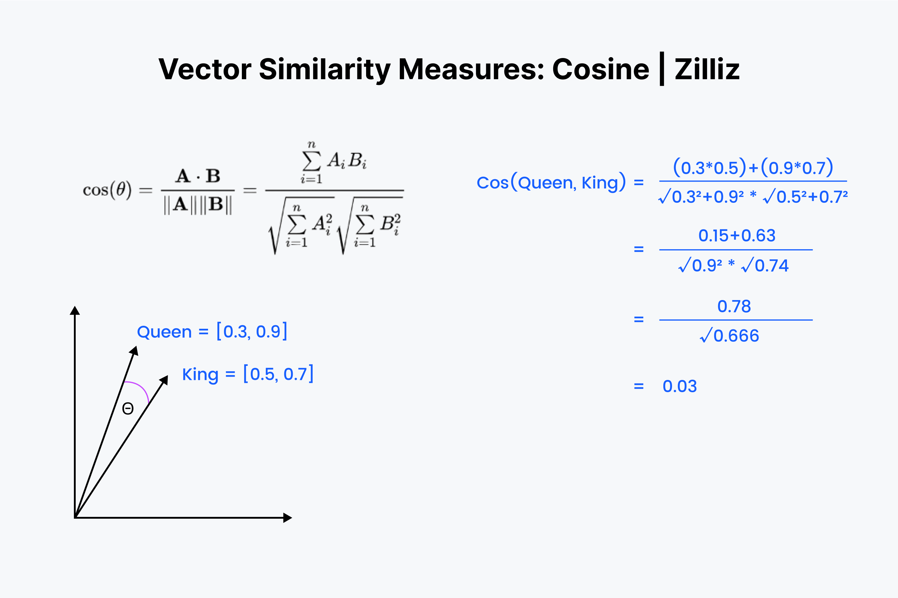
More formally, cosine similarity is calculated as:

sim(a,b) = (a·b) / (||a||·||b||)

Where a·b stands for the dot product, and ||a|| and ||b|| stand for the vectors’ lengths.

The cosine similarity ranges between -1 and 1:

1 means an angle of 0° (vectors are pointing in the same direction)
0 means a 90° angle (vectors are orthogonal)
-1 means a 180° angle (vectors are pointing in opposite directions)

When Should You Use Cosine Similarity?

Cosine similarity is primarily used in NLP applications. The main thing that cosine similarity measures is the difference in semantic orientation. If you work with normalized vectors, cosine similarity is equivalent to the inner product.

Cosine similarity is particularly useful when dealing with high-dimensional data, as it is computationally efficient and can handle sparse data. It’s ideal for solving semantic search and document classification problems since it allows you to compare the direction of the vectors (i.e., the overall content of the documents).

It’s probably not suitable when you have data where the magnitude of the vectors is important and should be taken into account when determining similarity. For example, it is not appropriate for comparing the similarity of image embeddings based on pixel intensities

Inner Product (Dot Product)

The inner product is the projection of one vector onto the other. The inner product's value is the vector's length drawn out. The bigger the angle between the two vectors, the smaller the inner product. It also scales with the length of the smaller vector. So, we use the inner product when we care about orientation and distance. For example, you would have to run a straight distance through the walls to your refrigerator.

How Does Inner Product Work?

The inner product should look familiar. It's just the first ⅓ of the cosine calculation. Line those vectors up in your mind and go down the row, multiplying downward. Then, sum them up. This measures the straight line distance between you and the nearest dim sum.

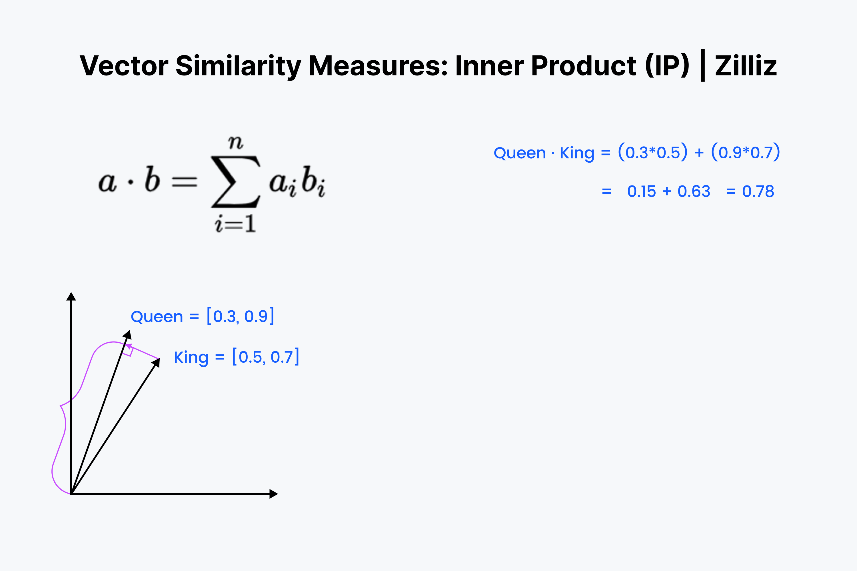
Mathematically, the dot product for vectors a and b is calculated as follows:

a·b = ∑(i=1 to n) aᵢbᵢ = a₁b₁ + a₂b₂ + a₃b₃ + … + aₙbₙ

The dot product can also be expressed as the product of the magnitudes of the vectors and the cosine of the angle between them:

a·b = |a|·|b|·cos(α)

The dot product is:

Positive if the angle between the vectors is less than 90 degrees
Negative if the angle between the vectors is greater than 90 degrees
Zero if the vectors are orthogonal (perpendicular)

When Should You Use Inner Product?

The inner product is like a cross between Euclidean distance and cosine similarity. When it comes to normalized datasets, it is the same as cosine similarity, so the inner product is suited for either normalized or non-normalized datasets. It is a faster option than cosine similarity, and it is a more flexible option.

You're likely to encounter many Large Language Models (LLMs) that use dot product for training. For example, the msmarco-bert-base-dot-v5 model on Hugging Face specifies the "suitable scoring functions" to be only dot product.

One thing to keep in mind with Inner Product is that it doesn't follow the triangle inequality. Larger lengths (large magnitudes) are prioritized. This means we should be careful when using IP with Inverted File Index or a graph index like HNSW.

In a recommender system based on collaborative filtering and matrix factorization, every user and every item (e.g., movie) has an embedding, and the model is learned such that the dot product between a user embedding and an item embedding is a good predictor of the rating that user will assign this item. If two products have embeddings with the same direction but different magnitudes, this can mean that the two products are about the same topic, but the one that has a larger magnitude is just better/more popular than the other.

Beyond the Basics: Additional Similarity Metrics

The three vector metrics mentioned above are the most useful regarding vector embeddings. However, they're not the only ways to measure the distance between two vectors. Here are some other ways to measure distance or similarity between vectors.

Manhattan Distance

Manhattan distance, also known as L1 distance, calculates the distance between points by summing the absolute differences across each dimension. Think of it as the distance a taxi would drive in a city with a grid layout (hence the name "Manhattan").

Unlike Euclidean distance which measures "as the crow flies," Manhattan distance follows the grid. This makes it advantageous in scenarios where outlier sensitivity needs to be minimized, as it doesn't square the differences like Euclidean distance does.

Manhattan distance is suitable for data with outliers and is commonly used in various applications including clustering and classification tasks.

Hamming Distance

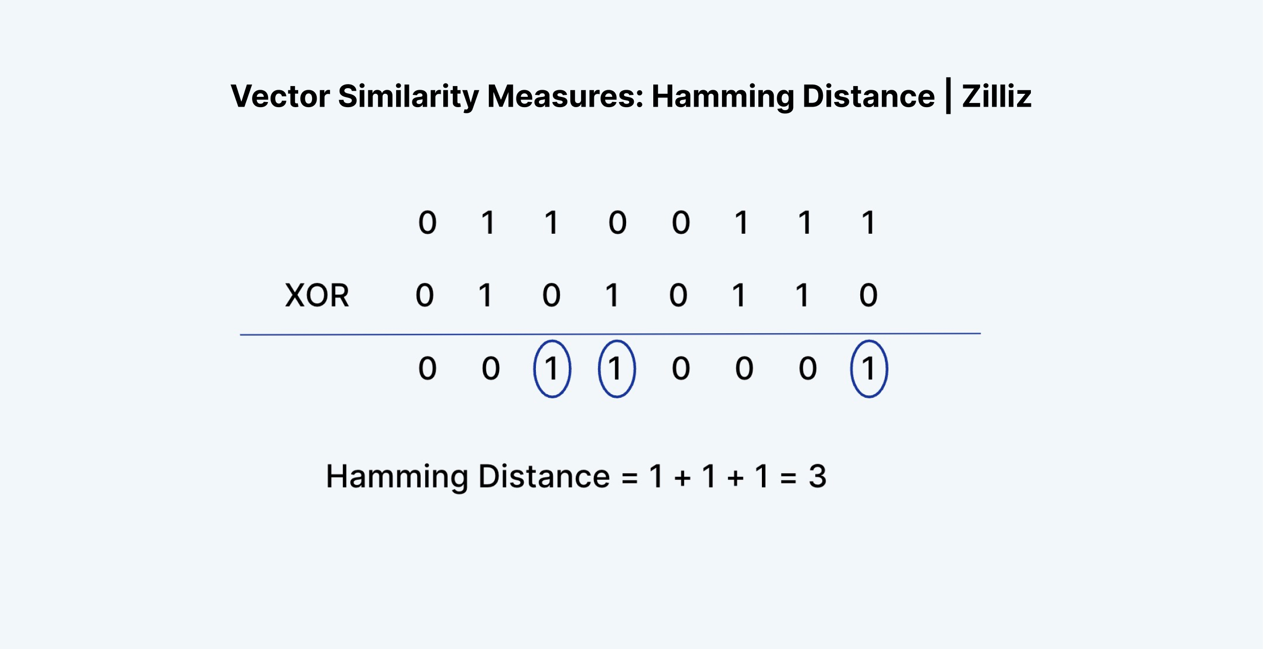
Hamming distance can be applied to vectors or strings. For our use cases, let's stick to vectors. Hamming distance measures the "difference" in the entries of two vectors. For example, "1011" and "0111" have a Hamming distance of 2.

In terms of vector embeddings, Hamming distance only really makes sense to measure for binary vectors. Float vector embeddings, the outputs of the second to last layer of neural networks, are made up of floating point numbers between 0 and 1. Examples could include [0.24, 0.111, 0.21, 0.51235] and [0.33, 0.664, 0.125152, 0.1].

As you can see, the Hamming distance between two vector embeddings will almost always come out to just the length of the vector itself. There are just too many possibilities for each value. That's why Hamming distance can only be applied to binary or sparse vectors—the type of vectors that are produced from a process like TF-IDF, BM25, or SPLADE.

Hamming distance is good to measure something like the difference in wording between two texts, the difference in the spelling of words, or the difference between any two binary vectors. But it's not good for measuring the difference between vector embeddings.

Here's a fun fact: Hamming distance is equivalent to summing the result of an XOR operation on two vectors.

Jaccard Index/Distance

Jaccard Distance

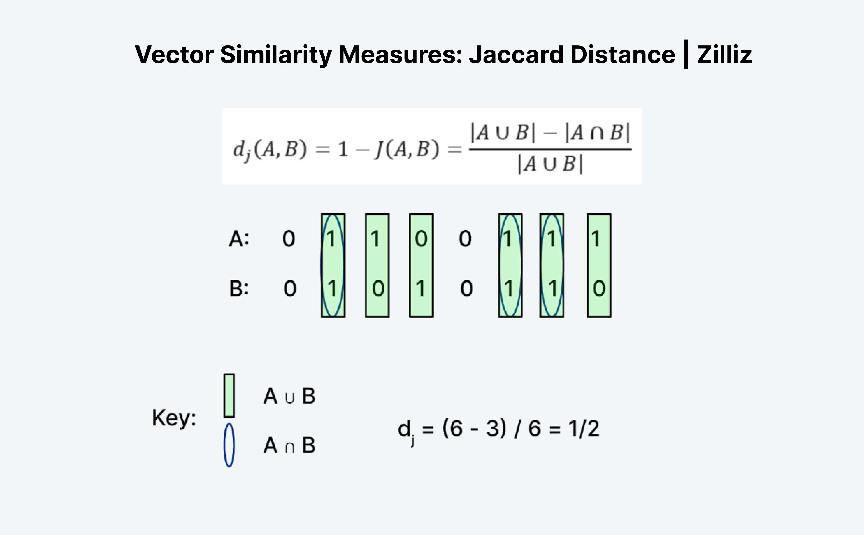
Jaccard distance is another way to measure two vectors' similarity or distance. The interesting thing about Jaccard is that there is both a Jaccard Index and a Jaccard Distance. Jaccard distance is 1 minus the Jaccard index, the distance metric Milvus implements.

Calculating Jaccard distance or index is an interesting task because it doesn't exactly make sense at first glance. Like Hamming distance, Jaccard only works on binary data. The traditional formation of "unions" and "intersections" can be confusing. A more intuitive way to think about it is with logic: It's essentially A "OR" B minus A "AND" B divided by A "OR" B.

We count the number of entries where either A or B is 1 as the "union" and where both A and B are 1 as the "intersection." For example, the Jaccard index for A (01100111) and B (01010110) is ½. In this case, the Jaccard distance, 1 minus the Jaccard index, is also ½.

Implementation Considerations

When implementing vector similarity search, there are several important considerations to keep in mind:

Vector Normalization

Normalization is the process of scaling vectors so they have a consistent scale, typically a unit length (magnitude of 1). This can be crucial when:

Using cosine similarity, as it focuses only on direction
Combining vectors from different sources with different scales
Wanting to make fair comparisons across different vector dimensions

The most common normalization approach is L2 normalization, where each vector is divided by its L2 norm (Euclidean length). After normalization, cosine similarity becomes equivalent to the inner product, which can improve computational efficiency.

Computational Efficiency

Different metrics have different computational costs:

Inner product is generally the fastest to compute
Cosine similarity requires normalization but can be optimized to use inner product
Euclidean distance involves more operations but can be optimized (like Milvus skipping the square root)

For large-scale applications, these efficiency considerations can significantly impact system performance and cost.

Integration with Vector Indexes

Vector indexes like HNSW (Hierarchical Navigable Small World), IVF (Inverted File Index), and ScaNN (Scalable Nearest Neighbors) are designed to accelerate similarity searches:

HNSW: Creates a navigable graph structure for efficient nearest-neighbor search. Works well with all similarity metrics but requires careful parameter tuning.

IVF: Divides the vector space into clusters, allowing searches to focus on relevant clusters. More efficient with metrics that follow the triangle inequality (like Euclidean distance).

ScaNN: Optimized for inner product search, making it excellent for recommendation systems and cases where dot product is the primary metric.

When selecting an index, consider both your similarity metric and the scale of your data. Some combinations (like inner product with IVF) require special attention due to mathematical properties.

Open-Source Contributions and Tools for Vector Similarity Search

The open-source community has made significant contributions to the field of vector similarity search, providing a variety of tools and libraries that facilitate efficient indexing and searching of large collections of vectors. Notable examples include Faiss, Annoy, and Hnswlib, which offer robust algorithms and data structures tailored for vector similarity search. These libraries are designed to handle the computational demands of high-dimensional vector spaces, making them invaluable for applications like recommendation systems and image retrieval. Additionally, frameworks such as TensorFlow and PyTorch provide comprehensive tools for building and training machine learning models that generate vector embeddings. The development of Approximate Nearest Neighbor (ANN) algorithms within these open-source projects has further enhanced the efficiency and scalability of vector similarity search, enabling faster and more accurate results.

Choosing the Right Metric for Your Application

Remember our rule of thumb: use the same similarity metric that was used to train your embedding model.

When choosing between metrics:

Use Euclidean distance when you care about the difference in magnitude. It's great for when your vectors have different magnitudes and you primarily care about how far your data points are in space.
Use Cosine similarity when you care about the difference in orientation. Perfect for NLP applications and scenarios where vector direction matters more than magnitude.
Use Inner product when you care about both magnitude and orientation. It's a versatile option that works well for both normalized and non-normalized datasets.
Use specialized metrics like Hamming or Jaccard for binary data or specific applications where these metrics are more appropriate.

If you don't know what similarity metric was used in the embedding model or if the vectors were created without a specific metric in the generation process, experiment with various similarity metrics to see what produces the best results for your specific use case.

Factors to Consider when Comparing Vectors

When comparing vectors, several critical factors must be considered to ensure accurate and meaningful results. The choice of distance metric is paramount, as it determines how similarity is quantified. Common distance metrics include Euclidean distance, which measures the straight-line distance between two vectors, cosine similarity, which assesses the angle between vectors, and dot product similarity, which considers both magnitude and direction. The dimensionality of the vector space also plays a crucial role; higher-dimensional spaces can capture more complex relationships but require more computational resources. Additionally, normalization of vectors is essential, particularly when using metrics like cosine similarity, as it ensures that comparisons are fair and consistent across different scales. By carefully considering these factors, you can optimize the performance and accuracy of your vector similarity search algorithms, leading to more relevant and insightful results.

Real-World Applications

Similarity metrics have numerous real-world applications in various fields:

Natural Language Processing: Cosine similarity shines in text classification, sentiment analysis, and information retrieval tasks. The semantic orientation that cosine similarity measures makes it ideal for comparing document content regardless of length.

Recommendation Systems: Whether you're recommending products, movies, or friends on social media, similarity metrics are the backbone of these systems. Euclidean distance can measure absolute differences in user behavior, while inner product can predict user ratings in collaborative filtering models.

Image and Video Analysis: For image similarity, classification, and object detection, metrics like Euclidean distance and Manhattan distance play crucial roles in measuring visual similarity.

Clustering and Classification: Grouping similar data points together relies heavily on appropriate similarity metrics. The choice between Euclidean, cosine, or other metrics can dramatically affect the quality of your clusters.

Conclusion and Future Trends

In this post, we learned about the most useful vector similarity search metrics: L2 (Euclidean) distance, cosine similarity, and inner product, as well as specialized metrics like Hamming distance and Jaccard index. Each of these has different use cases:

Euclidean is for when we care about the difference in magnitude
Cosine is for when we care about the difference in orientation
Inner product is for when we care about both magnitude and orientation
Specialized metrics serve specific purposes with binary or sparse data

Understanding the characteristics and limitations of each similarity metric is essential to choose the most appropriate one for a specific task. By selecting the right similarity metric, we can improve the accuracy and relevance of our results, leading to better decision-making and insights.

As vector embeddings continue to evolve with more sophisticated models, we can expect new similarity metrics to emerge that better capture the nuances of specific domains. The increasing prominence of multimodal embeddings—combining text, image, audio, and more—will likely drive innovation in how we measure and compare vector similarity across different modalities.

So yes, it turns out you can compare apples and oranges after all—you just need the right vector embedding and similarity metric to do it!

Check these videos to learn more about Vector Similarity Metrics, or read the docs to learn how to configure these metrics in Milvus.

Updated on Apr 07, 2025

Yujian Tang
Yujian Tang is a Developer Advocate at Zilliz. He has a background as a software engineer working on AutoML at Amazon. Yujian studied Computer Science, Statistics, and Neuroscience with research papers published to conferences including IEEE Big Data. He enjoys drinking bubble tea, spending time with family, and being near water.

Content

Start Free, Scale Easily

Try the fully-managed vector database built for your GenAI applications.

Try Zilliz Cloud for Free

Share this article

Keep Reading

ColPali + Milvus: Redefining Document Retrieval with Vision-Language Models

When combined with Milvus's powerful vector search capabilities, ColPali becomes a practical solution for real-world document retrieval challenges.

Vector Databases vs. Graph Databases

Use a vector database for AI-powered similarity search; use a graph database for complex relationship-based queries and network analysis.

Top 10 AI Agents to Watch in 2025 🚀

AI agents are like having a supercharged assistant by your side—analyzing data, making decisions, and seamlessly integrating with tools and environments.