Learn
Large Language Models (LLMs) 101

RouteLLM: An Open-Source Framework for Navigating Cost-Quality Trade-Offs in LLM Deployment

Nov 28, 202415 min read

RouteLLM is an open-source framework that enables developers to efficiently route tasks to the most suitable LLMs based on cost, latency, and accuracy.

By Ruben Winastwan

Read the entire series

The popularity and hype surrounding Large Language Models (LLMs) in AI cannot be denied today. Their versatility makes LLMs particularly attractive to be implemented across various industries and use cases. Fortunately, there is a wide array of LLMs available, such as ChatGPT, Claude, Mistral, Llama, Qwen, and many others. On top of that, developers of these LLMs frequently launch several variants within a single model family to provide more options. For example, Meta has released the Llama 3.2 model in four different variants: 1B and 3B text-only LLMs, as well as 11B and 90B vision LLMs.

The sheer number of LLMs available can make it challenging to select the best model for our specific use case. In many scenarios, we will likely need to utilize more than one LLM to balance cost with response quality. Therefore, it would be beneficial to have the flexibility to choose different LLMs that optimize cost and response quality based on the complexity of the query. In this article, we will discuss a method called RouteLLM that can help us to implement this concept. So, without further ado, let’s get started.

What is RouteLLM?

RouteLLM is an open-source framework designed to simplify the deployment and management of large language models (LLMs) in production. It enables developers to efficiently route tasks to the most suitable LLMs based on factors like cost, latency, and accuracy. With support for multiple LLM providers, including OpenAI, Anthropic, and open-source models like Falcon and LLaMA, RouteLLM ensures seamless integration and scalability. Key features include intelligent routing, dynamic provider selection, and task optimization. By offering flexibility and reducing complexity, RouteLLM is ideal for organizations looking to leverage multiple LLMs effectively in diverse applications.

Motivations Behind RouteLLM

One of the most common constraints of using LLMs in real-life scenarios is the cost. Despite being really powerful in solving a wide variety of tasks, we know that implementing LLMs can be expensive, regardless of whether we use closed-source or open-source models.

If we use closed-source models like ChatGPT or Claude, the cost depends on factors such as the number of queries, the number of tokens in a query, and the number of generated tokens. Meanwhile, if we use open-source models like Llama, Mistral, or Qwen, the cost depends on factors such as the type and number of GPUs, as well as the time needed for the LLM to serve the queries.

The rule of thumb is that the larger the size of an LLM, the more expensive its operation cost will be. However, the size of an LLM also normally corresponds to its capabilities. The larger the size of an LLM, the higher its response quality will be. Therefore, we are faced with a trade-off scenario between performance and cost. Choosing a large LLM will almost guarantee us a high-quality response even when the query is complicated, but it comes with a high cost. The opposite applies if we choose a smaller LLM.

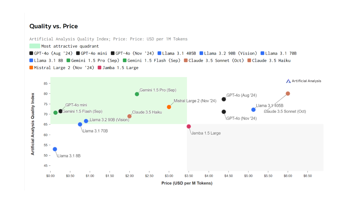Figure- Cost-quality comparison between different LLMs..png

Figure: Cost-quality comparison between different LLMs. Source.

Of course, we can choose a large LLM to ensure the response quality of all queries. However, using a large LLM to generate responses for all queries would be a waste of money because not all queries are complicated. If we have a simple query, a smaller model would be sufficient to generate a high-quality response, and we can save money from this.

To solve this problem, we can implement a method to classify the complexity of a query. Then, based on the classification result, we choose the appropriate LLM to generate the response. If the method classifies a query as "complicated", then the method will send this query to the large, expensive LLM. Meanwhile, if a query is classified as "simple", the query will be sent to the small, cheap LLM.

RouteLLM is one of the methods that implement this idea. In this method, each query is first processed by a so-called routing function. This routing function decides which LLM to route the query to with the objective of optimizing the quality of responses while minimizing cost. However, developing a robust routing function is not trivial, as it needs to infer the complexity and domain of the query as well as understand candidate LLMs' capabilities before routing the query. In the next section, we'll discuss how RouteLLM tackles these challenges.

The Fundamental of RouteLLM

The concept of LLM routing in general is simple: given N different LLMs, a routing function's task is to classify which LLM a query q should be routed to. Therefore, the final output of a routing function should be a vector with a dimension of N, where each element n corresponds to some sort of probability of q being routed to LLM n.

In order to find the best LLM to generate the response for a query q, the routing function needs to be trained to maximize the response quality while optimizing the cost. Therefore, the training data of a routing function normally has the structure of (q, l_i,j), where q represents the query and l_i,j is the label obtained after comparing the responses of LLM i and j on query q.

Figure- Visualization of LLM Routing in general..png

Figure: Visualization of LLM Routing in general.

RouteLLM is a routing method that follows the above concept. Specifically, its routing function has been trained to classify the complexity of a query and route it to either the strong model or weak model. The strong model here refers to the advanced closed-source LLM with a huge number of parameters, while the weak model normally contains fewer parameters and is open-source. Since we're only dealing with two different LLMs, the routing problem in RouteLLM is commonly called binary routing.

There are two main components implemented by RouteLLM to train the routing function: win prediction model and cost threshold.

Win prediction model: predicts the probability of the strong model winning the binary routing. The output of the router model is then a vector with two elements: one represents the winning probability of the strong model, while the other represents the winning probability of the weak model.
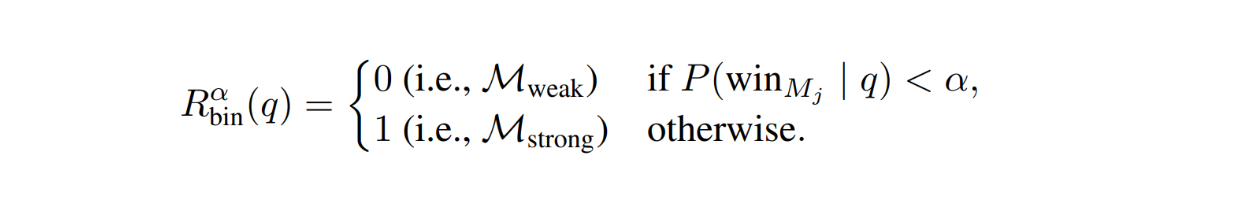
Cost threshold: converts the routeing function output into a routing decision. For each query q, the routing decision is defined with the following formula:

equation .png

where α is the threshold value that controls the trade-off between response quality and cost. The higher the threshold value, the stricter we are with the cost, which forces the routing function to prioritize cost over response quality.

During the inference time, the response to a query q is then generated by either the strong model or weak model, depending on the decision from the routing function.

The Training Process of RouteLLM

As mentioned in the previous section, the main gist of RouteLLM is to train a routing function for query routing in a binary classification problem. However, as with any machine learning problems out there, we need to gather the data first before the training process.

The training data for RouteLLM has the following format: {q, M_s, M_w, l_s,w}, where q is the query, M_s is the response from the strong model, M_w is the response from the weak model, and l_s,w is the label that represents the response preference between two models from human judgment.

Training Data Gathering Process

To gather the training data, the author of RouteLLM implemented several data-gathering techniques.

The first one uses 80K data gathered from the online Chatbot Arena platform. This data source contains the query, the responses of two anonymous LLMs, and the preference result between two responses from the users who act as the label.

However, since the two compared models are random, the percentage of available labels between any two models is less than 0.1%. To solve this problem, the author implemented a clustering of models into 10 tiers based on their Elo score on the Chatbot Arena leaderboard. The higher the tier, the stronger the model is. Below is the visualization of these tiers:

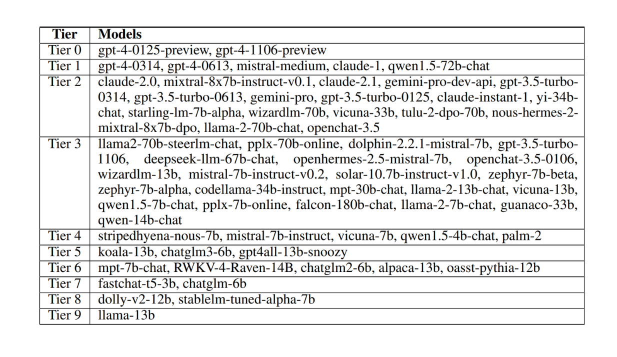Figure- Clustering of LLMs into 10 tiers on the Chatbot Arena dataset..png

Figure: Clustering of LLMs into 10 tiers on the Chatbot Arena dataset. Source.

For the training of the routing function, the author took the models in the first tier as the strong model and the models in the third tier as the weak model. It's also important to note that the author didn't use the original responses from the Chatbot Arena platform to represent M_s and M_w, but rather regenerated the responses based on the given query.

To improve the generalization of the routing function during training, the author also performed a couple of data augmentation methods:

Golden-labeled dataset: this dataset is gathered from multiple-choice queries, so we can judge and compare the responses of any two LLMs objectively. To perform this data augmentation, the author took 1.5k questions from the validation set of the MMLU dataset and derived the label l_s,w based on the responses from the two LLMs.
LLM-judge-labeled dataset: one common way to get a preference label is by using another strong LLM as a judge to derive the comparison label l_i,j given the responses of two LLMs. To perform this data augmentation, the author used the Nectar dataset. This dataset contains a collection of queries with the corresponding responses from several models. The author picked a total of 120K queries, selecting the responses of the corresponding queries from the chosen strong and weak models, and used GPT-4 as a judge to derive the comparison label l_s,w.

RouteLLM implements four different approaches to optimizing the routing function: similarity-weighted (SW) ranking, matrix factorization, BERT classifier, and causal LLM classifier. Let's discuss SW ranking first.

First Routing Approach - SW Ranking

The idea of SW ranking is to rank the two models (strong and weak models) based on how likely they are to be the best at answering a specific user query. For each query in the training set q_i, a similarity score (S(q, q_i)) is calculated to measure how similar q_i is to the new user query q. The intuition is that more similar training queries should have more influence on the ranking. A weight ω_i is assigned to each training query q_i, based on its similarity to the current query q.

Since we're calculating the similarity between queries, the query needs to be transformed into embeddings first. To do this, the embedding model called text-embedding-3-small from OpenAI was used.

Next, a Bradley-Terry (BT) model is implemented. This model estimates the probability that the strong model will win over the weak model based on their scores. This corresponds to the win prediction model mentioned in the previous section, and this BT model estimates the probability of the strong model winning with the following formula:

SW Ranking - equation.png

As you can see, the BT model relies on coefficients ξ_s (coefficient of strong model) and ξ_w (coefficient of weak model). These coefficients are learned using a binary cross-entropy loss function during training. The weights of each query will also influence how much each training query affects the learning process.

SW Ranking - equation 2.png

During the inference time, when the user provides a new query, there's no need to retrain the model. The ranking is computed on the fly and the probability of the strong model winning can be calculated using the learned coefficients using the formula presented above.

Second Routing Approach - Matrix Factorization

The second method draws inspiration from matrix factorization commonly used in recommendation systems. The main goal is to optimize a hidden scoring function s(M,q) which assigns a score to a model when it answers a query q. This score reflects how well the model performs on that query. If the strong model M_s performs better than the weak model M_w, the scoring function should ensure:

Matrix Factorization - equation.png

Therefore, to ensure the relationship above, the winning probability of the strong model is modeled with the following formula:

Matrix Factorization - equation 2.png

where σ is the sigmoid function.

If this method is quite difficult to understand, just imagine a table with two rows and many columns. The rows represent the models being compared, the columns represent queries, and each cell represents how well a model does on a query. This method tries to fill in the cells in the table by learning the patterns from given data using a combination of model and query representations.

Third Routing Approach - BERT Classifier

This method utilizes BERT to predict the win probability of the strong model for a given query q. The win probability is modeled with the following formula:

BERT Classifier - equation.png

As you might already know, BERT is a model that uses several stacks of Transformer encoders under the hood. For each input query q, BERT processes it by prepending a special token [CLS] in the first position of the query and produces a numerical feature for each token with a specific dimension

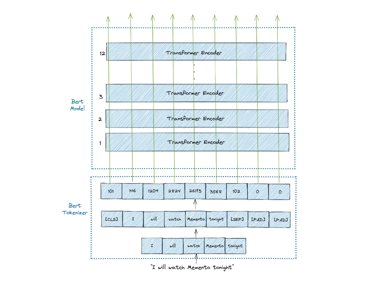Figure- BERT architecture..png

Figure: BERT architecture.

The approach takes only the numerical feature of the [CLS] token and then feeds it into a logistic regression head to optimize the modeling probability.

Fourth Routing Approach - Causal LLM Classifier

This method utilizes Llama 3 8B as a classifier to evaluate model performance. Specifically, the win probability of the strong model performing better than the weak model is determined by using an instruction-following concept.

The user query is formatted into an instruction prompt (e.g., "Compare models Ms and Mw on query q. Which one wins?"). The model reads this prompt and predicts an output directly as tokens. In addition, the comparison labels are added to the model's vocabulary, so it can generate output with a similar structure as the labels.

RouteLLM Metrics

Once the routing function has been trained with the four approaches mentioned above, we need to test the performance of each approach. To quantify the performance of each routing function, RouteLLM implemented several different metrics.

The first metric is the percentage of calls to the strong model. This metric is useful to quantify the cost efficiency:

RouteLLM Metrics - equation.png

To optimize the cost, we normally want this metric to be as low as possible.

The second metric is the average response quality on an evaluation dataset. As the name suggests, this metric quantifies the overall quality of the responses using the routing function. Ideally, we want the score of this metric to be as high as possible.

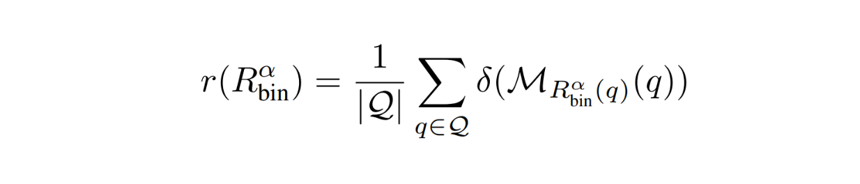RouteLLM Metrics - equation 2.png

Since we're using a routing function, the response quality will be somewhere between the quality of the weak model as the lower bound and the strong model as the upper bound. Therefore, the author also defined a metric called performance gap recovered (PGR) that quantifies the router's performance relative to the performance gap between both models:

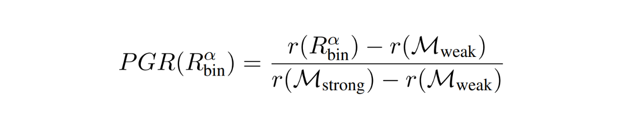RouteLLM Metrics - equation 3.png

However, there is one big problem with the metric above. If our queries are very simple and our router always directs our queries to the strong model, then the PGR metric will always be 1. The solution is to quantify PGR repeatedly with different cost threshold alpha values. Therefore, we get the average PGR of our routing function given various cost constraints.

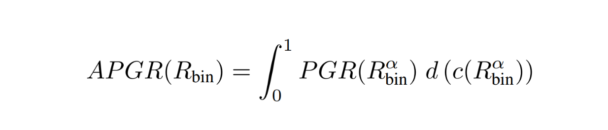RouteLLM Metrics - equation 4.png

Figure- Routing performance:cost trade-off between GPT-4 and Mixtral-8x7B..png

Figure: Routing performance/cost trade-off between GPT-4 and Mixtral-8x7B. Source.

One important metric that we also need to quantify is the cost required to achieve a certain level of performance. As you already know, the main goal of RouteLLM is to optimize the response quality while minimizing the cost. To capture this, the author defined a metric called call-performance threshold (CPT).

As you can see in the visualization image above, given a desired performance level (50% PGR), the CPT quantifies the minimum number of calls to the strong model required to achieve the desired PGR, which in the visualization corresponds to 37%.

Experiment Results

To test the performance of routing functions after training with the four different methods in the previous section, several datasets were used, including the validation set of Chatbot Arena, MMLU, MT Bench, and GSM8K.

The GPT-4-1106-Preview model was used as the strong model, and Mixtral 8x7B model was used as the weak model during testing. In each benchmark dataset, the routing functions are compared with each other and a random baseline. The random baseline represents the routing function where it randomly routes queries under a specific cost constraint.

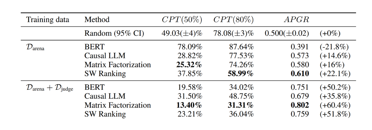Figure- RouteLLM results on MT Bench.png

Figure: RouteLLM results on MT Bench. Source.

As you can see, the routing functions trained on Arena and LLM-judge-labeled dataset with BERT, matrix factorization, and SW ranking approaches performed the best on the MT Bench dataset. They achieved almost 50% fewer GPT-4 calls to reach CPT(80%) compared to the random baseline.

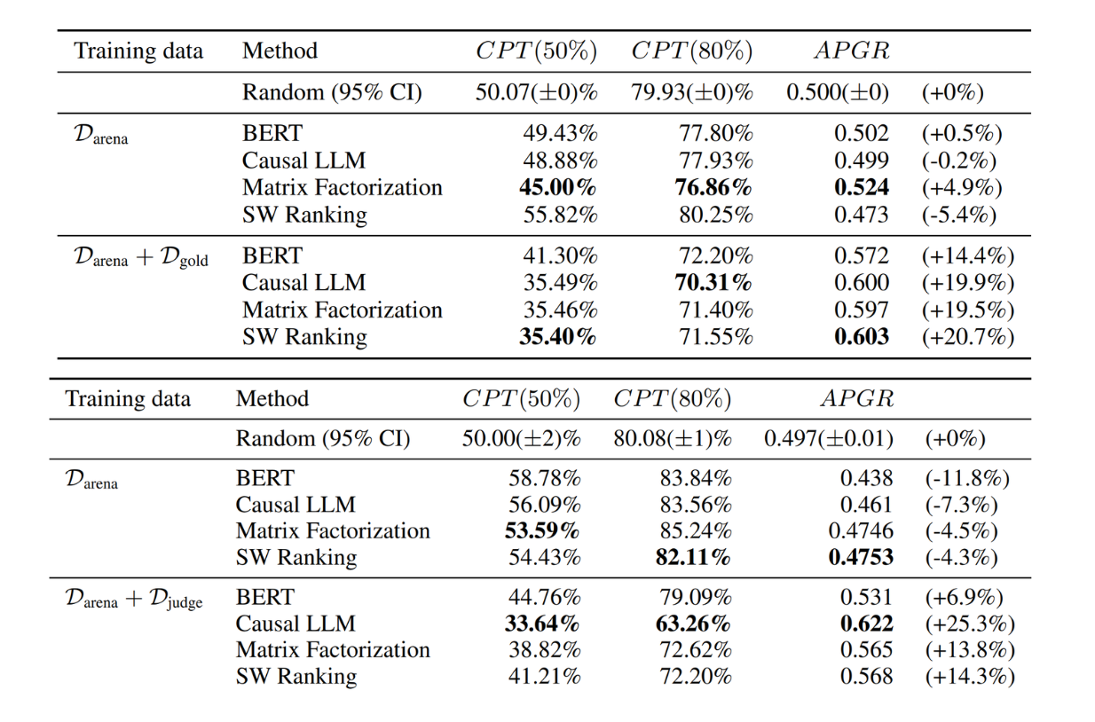Figure- RouteLLM results on MMLU (top) and GSM8K (bottom)..png

Figure: RouteLLM results on MMLU (top) and GSM8K (bottom). Source.

Meanwhile, on the MMLU and GSM8K datasets, all routing functions trained on the Arena dataset performed poorly compared to the random baseline, simply because the datasets are completely different from the training data. However, when we use the routing functions trained with both Arena and augmented datasets, the performance of all routing functions improved.

What's important to note is that the augmented datasets contained only small fractions of the overall training data. This shows that we can fine-tune the routing functions even with a small number of samples.

In the above results, we used GPT-4 as the strong model and Mixtral 8x7B as the weak model. What if we use different combinations of strong and weak models? To test this, the author also tested different combinations of strong and weak models without retraining the routing function. Specifically, the author used Claude 3 Opus as the strong model and Llama 3 8B as the weak model and tested the routing function on the MT Bench dataset.

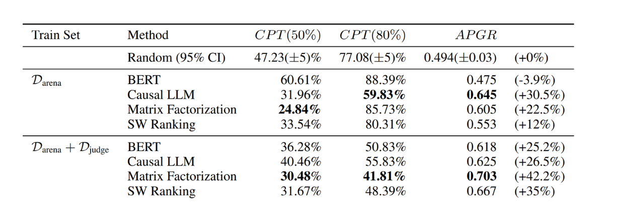Figure- RouteLLM results on MT Bench with Claude 3 Opus and Llama 3 8B. .png

Figure: RouteLLM results on MT Bench with Claude 3 Opus and Llama 3 8B. Source.

As you can see, the routing functions still achieved good results even when the model pair was replaced. The performance of this new model pair is also comparable with the original model pair, showing the generalization property of RouteLLM without additional training.

With GPT-4 as the strong model and Mixtral 8x7B as the weak model, RouteLLM managed to save costs approximately 3.66x compared to the random baseline on the MT Bench with CPT 50%, and 2.49x with CPT 80% by making efficiently fewer calls to GPT-4

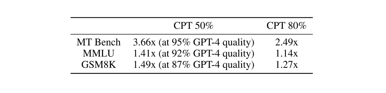Figure- Cost saving ratio of the best performing routers over GPT-4..png

Figure: Cost saving ratio of the best performing routers over GPT-4. Source.

Conclusion

In this article, we have discussed RouteLLM, a method that provides a solution to the cost-quality trade-offs when using LLMs in production. By intelligently routing queries between a strong model and a weak model based on complexity, RouteLLM optimizes the balance between high response quality and operational cost. Its various routing approaches, such as SW Ranking, Matrix Factorization, BERT-based classification, and causal LLM classification demonstrated flexibility and adaptability across datasets and model combinations.

From the experimentation results, RouteLLM showed its efficiency compared to a random router in reducing the reliance on expensive LLMs while maintaining high-quality responses. This, in turn, allows us to save the cost when using LLM in production.