Learn
Large Language Models (LLMs) 101

LoRA Explained: Low-Rank Adaptation for Fine-Tuning LLMs

Nov 14, 202414 min read

LoRA (Low-Rank Adaptation) is a technique for efficiently fine-tuning LLMs by introducing low-rank trainable weight matrices into specific model layers.

By Ruben Winastwan

Read the entire series

Fine-tuning is the go-to approach to optimizing the performance of any deep learning model on a downstream task. Let's say we would like to leverage the powerful performance of the BERT model for a text classification task. Although BERT has been trained on a large amount of data and has achieved state-of-the-art performance on many benchmark datasets, its performance might be suboptimal when applied to our specific dataset. In this case, fine-tuning can help optimize the BERT model's performance on our dataset.

However, as the size of the model we need to fine-tune grows, implementing the traditional fine-tuning approach becomes increasingly challenging. This is where LoRA comes in.

LoRA (Low-Rank Adaptation) is a technique for efficiently fine-tuning large language models (LLMs) by introducing low-rank trainable weight matrices into specific model layers. It enables us to fine-tune large models, even those with tens of billions of parameters. In this article, we'll discuss what LoRA is and how it works. Let's first explore why we need LoRA in the first place.

The Problems with Traditional Fine-Tuning Approaches

Traditional fine-tuning approaches are simple: given a pre-trained model and a labeled domain-specific dataset, we train the model on this specific dataset. Therefore, you can think of the fine-tuning process as training a machine learning model in a supervised manner. However, during fine-tuning, the dataset size doesn't have to be huge, as we only want to update the weights of a pre-trained model according to our data.

Figure- Fine-tuning workflow.png

Figure: Fine-tuning workflow

As the process of fine-tuning is essentially the same as supervised training of a machine learning model, the fine-tuning speed depends on at least three factors: the hardware specification (the GPU we use), the size of the domain-specific dataset, and the number of parameters in the model. Assuming we've fixed the hardware specification and dataset size, the fine-tuning process primarily depends on the model size: the more parameters the model has, the longer it takes to fine-tune.

This wouldn't be a big deal if we worked with a small to medium-sized deep learning model. However, if we're trying to fine-tune an LLM with billions of parameters, the process becomes very expensive in terms of both computation and cost. Therefore, a solution is needed to make the fine-tuning process more efficient, especially when dealing with LLMs, which are highly relevant nowadays.

Also, as mentioned previously, the main purpose of fine-tuning is to optimize a model's performance on our specific dataset. Once we've fine-tuned a model, its performance will be good if it has to predict unseen data with a similar distribution to the dataset used during fine-tuning. However, if we have unseen data that deviates significantly from the fine-tuning dataset, then the predictions from the model would be unreliable. In this case, we must re-tune the model to the new domain-specific dataset.

Now imagine if we have two unrelated domain-specific use cases. This means we will most likely end up with two models, each fine-tuned on one specific use case. This would be fine if the size of our base pre-trained model is not that large. However, if we're working with LLMs, storing several versions of the same LLM, each fine-tuned with a specific dataset, is highly inefficient in terms of memory management and storage.

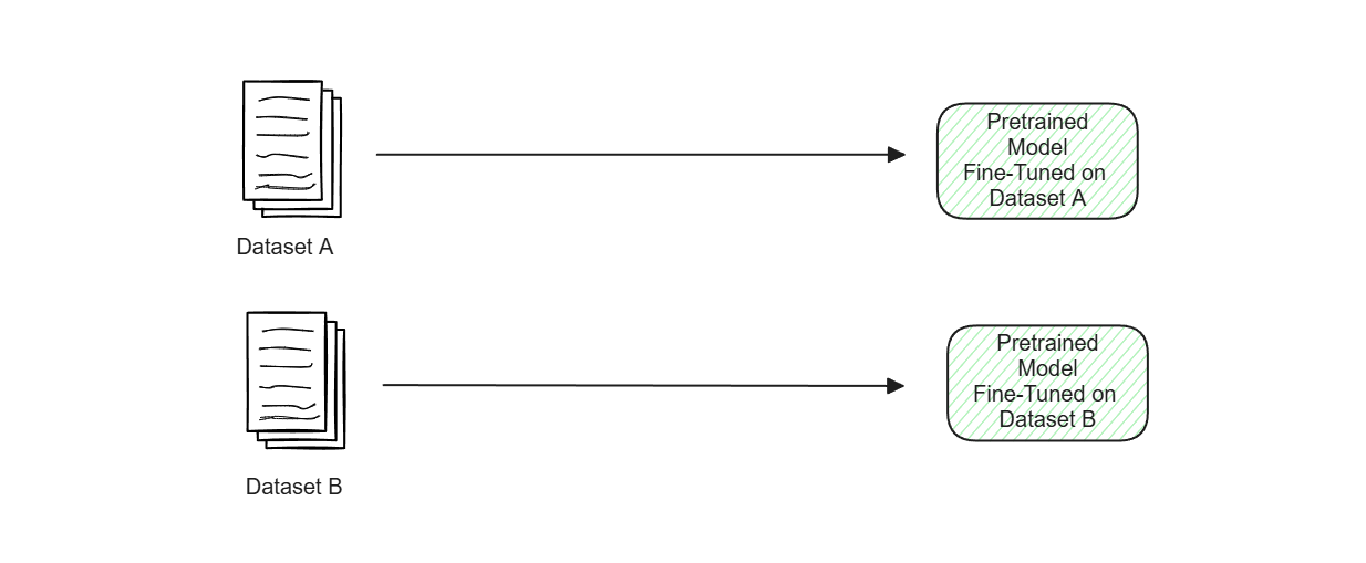Figure- Two versions of the same pretrained model fine-tuned on two domain-specific datasets..png

Figure: Two versions of the same pretrained model fine-tuned on two domain-specific datasets.

Therefore, we need a better way to store several versions of the same model, each fine-tuned on specific data. In the next section, we'll discuss several approaches to tackle these problems.

The Concept of Adapters and Prefix Tuning

Before the introduction of LoRA, several methods were proposed to solve the problems related to the traditional fine-tuning approach mentioned above. The first one is the bottleneck adapter approach introduced by Houlsby et al. in 2019.

The concept of bottleneck adapters is simple. Before the fine-tuning process, we freeze the weights of the pretrained model. Then, we introduce a collection of small, trainable parameters inside the layers of the pretrained model called adapters. During fine-tuning, we update only these adapters instead of the whole weights of the pretrained model. This approach makes the fine-tuning process much faster than the traditional approach, as we don't need to calculate the gradient of the whole model's weights and update them in each iteration.

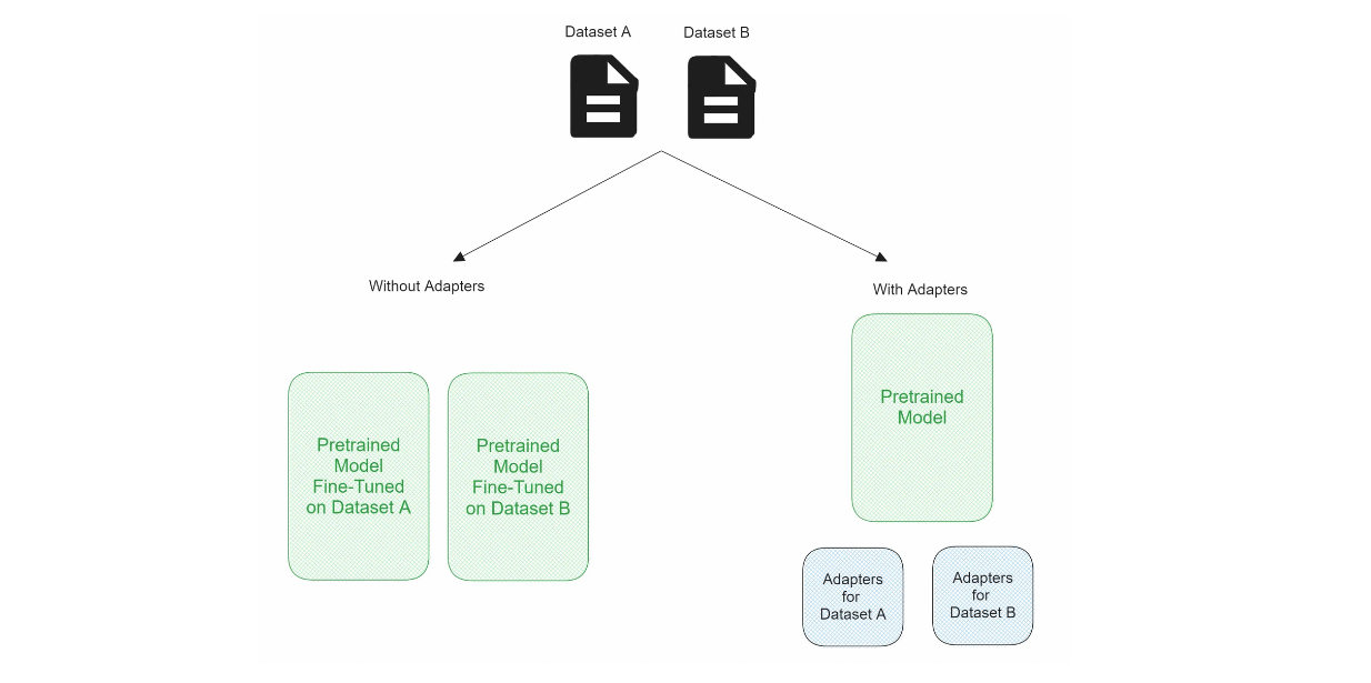Figure- Comparison between normal fine-tuning vs fine-tuning with adapters..png

Figure: Comparison between normal fine-tuning vs fine-tuning with adapters.

Moreover, these adapters can be easily removed and inserted back into the pretrained model. This is another advantage of using adapters since if we have several domain-specific use cases, we don't need to store several versions of fine-tuned models, but rather one pretrained model and several adapters. Depending on the use case, we can then plug these adapters into the pretrained model during inference.

In the bottleneck adapter introduced by Houlsby, the adapter consists of two normal dense layers, with an activation function in between. The first dense layer downscales the input, while the second dense layer upscales the output, hence the name "bottleneck."

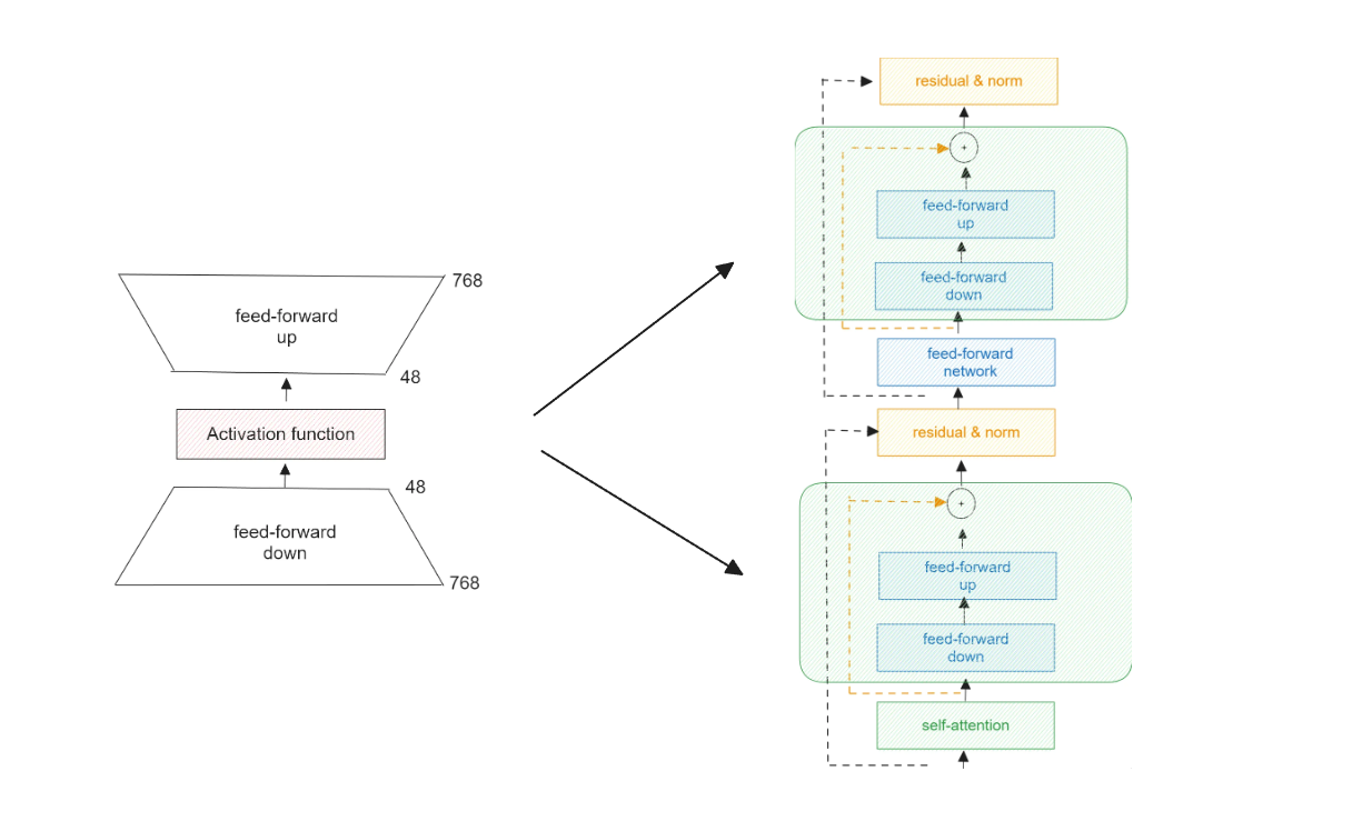Figure- Bottleneck adapter and its placement in a Transformer layer in Houlsby configuration..png

Figure: Bottleneck adapter and its placement in a Transformer layer in Houlsby configuration.

These bottleneck adapters are placed inside the model with Transformer-based architecture. In the Houlsby configuration, they're placed after the multi-head attention and the dense layers inside each Transformer layer.

Aside from the Houlsby configuration, there are other popular configurations: Lin, Pfeiffer, and AdapterDrop. The configurations in Lin and Pfeiffer setups are very similar: the adapters are placed after the dense and normalization layers inside each Transformer layer. Meanwhile, AdapterDrop is another approach to improve the efficiency of the method by dropping the adapters in some of the Transformer layers.

The main problem with adapters is that there is no easy way to bypass the extra computation step they introduce. This means that the model with these adapters can only be processed sequentially, resulting in a noticeable increase in latency during model inference.

Another solution aside from the application of adapters is prefix tuning. In prefix tuning, a small set of parameters, known as "prefixes," are introduced. Prefixes are learnable embeddings, often initialized randomly or based on task-specific information. They act like additional prompts or context that can guide the model to perform better on new tasks.

The core idea of prefix tuning is the same as adapters. We freeze the weights of a pretrained model and only update the embeddings of the prefixes so that they can learn to generate task-relevant embeddings that condition the output of each layer.

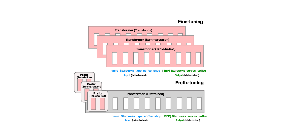Figure- Normal fine-tuning (top) vs prefix fine-tuning (bottom). .png

Figure: Normal fine-tuning (top) vs prefix fine-tuning (bottom). Source.

However, there are at least two drawbacks to prefix tuning. First, it's very difficult to optimize. Second, we need to reserve some chunks of the model's sequence length for these prefixes in advance. This, in turn, reduces the sequence length available to process a downstream task, which might negatively affect the overall performance of the model after the fine-tuning process.

LoRA has been introduced to solve all of the challenges mentioned above, and we'll talk about its concept in the next section.

The Concept of LoRA and How It Works

Before discussing how LoRA works in detail, we first need to understand how the model's weights are updated during a normal fine-tuning process.

As the fine-tuning process is similar to supervised training methods, the weights of the model are updated by modifying the weights from the previous iteration with the gradient of the weights in the current iteration. The gradient of each weight tells us how much a weight needs to be adjusted to get the model to predict the training data correctly. The equation to update the weights in each iteration during the fine-tuning process looks like this:

equation 1.png

where W_current is the weights of the current iteration, W_previous is the weights of the previous iteration, 𝜂 is the learning rate, and ∇W is the gradient of the weights. To make everything simpler, the weight updating process after fine-tuning can be summarized with the following formula:

equation 2.png

where W is the final fine-tuned weights, W₀ is the original weights of a pretrained model, and ΔW is the adjustment that needs to be made to each weight after the fine-tuning process. For illustration purposes, let's say that our model has 9 parameters, hence 9 weights. We can see the weight updating process in the form of two matrices as shown below:

Figure- Weight updating process after fine-tuning in the form of two matrices..png

Figure: Weight updating process after fine-tuning in the form of two matrices.

As you can imagine, the larger the model, the more parameters it has. If the model has more parameters, the matrices will be larger, and therefore, the computational cost will also be higher.

Each matrix has a rank. The rank of a matrix represents the maximum number of linearly independent rows or columns in the matrix. Taking an example of the 3x3 weight matrix visualized above, let's say for each row and column, we have values like below:

Figure- Example of a linearly dependent column (column 3 is linearly dependent to column 1)..png

Figure: Example of a linearly dependent column (column 3 is linearly dependent to column 1).

We can say that column 3 of the matrix is linearly dependent on column 1, as we can get column 3 by multiplying each row in column 1 by 5. Therefore, the rank of our matrix is 2.

The hypothesis in LoRA is that if we somehow remove the linearly dependent columns (column 3 in our case) from the matrix, we essentially reduce the dimension of the matrix without losing too much information from the original matrix. Thus, in LoRA, we don't need to optimize the full-rank, large weight matrix with high dimensionality, but rather we decompose the full rank weight matrix into its low-rank adaptations. If our full rank original matrix has a dimension of d x k, then we can decompose it into two low-rank adaptations with matrices d x r and r x k, where r is the rank. r is the hyperparameter that we need to choose in advance.

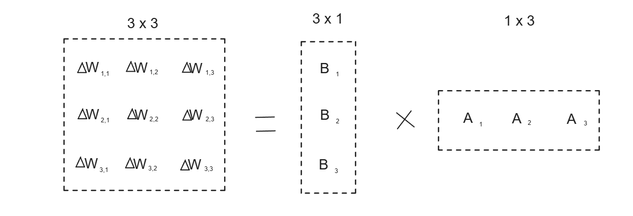Figure- Matrix decomposition into its low-rank adaptation

Figure: Matrix decomposition into its low-rank adaptation.

Based on the illustration above, we choose the rank of decomposition to be 1. As you can see, we should get a performance gain during fine-tuning computation because we store fewer parameters to update the original weights (from 9 in the original matrix to 3 in matrix A + 3 in matrix B). As you can imagine, the larger the dimension of the original matrix, the higher the performance gain we get by decomposing it into its low-rank adaptation.

However, we need to pay attention to the value of r that we choose. If we choose r to be too low, then we'll lose a lot of information from the original matrix. The weight updating process during the fine-tuning process follows the following formula:

equation 3.png

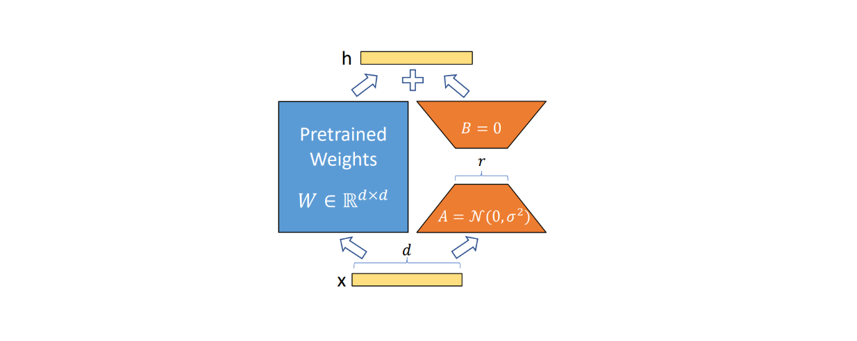Figure- LoRA fine-tuning workflow. .png

Figure: LoRA fine-tuning workflow. Source.

where W is the updated weights, W₀ is the original pretrained weights, and A and B are the low-rank decomposition of ΔW.

The result of B.A is also then scaled by α/r. We normally set the value of α equal to the first r value that we test if we decide to test several r values during the fine-tuning process.

Unlike bottleneck adapters, LoRA doesn't introduce additional latency during inference time as we can explicitly update the weights of the model for a specific domain-specific task with W = W₀ + BA. When we need to switch to another domain-specific task, we can recover the original pretrained weights W₀ by subtracting BA and then adding a different B’A’ to W₀. We also don't need to reserve additional space in the sequence like in prefix tuning to fine-tune a model.

Experimentation Results with LoRA

To compare the performance of LoRA with other methods like Adapters and Prefix tuning, the authors of the paper tested several deep learning models fine-tuned with all of these methods on several benchmark datasets.

Specifically, the authors fine-tuned RoBERTa, DeBERTa, and GPT-2 models with the normal fine-tuning approach (FT), adapters with configurations from Houlsby (Adpt H), Lin (Adpt L), Pfeiffer (Adpt P), AdapterDrop (Adpt D), Prefix-embedding tuning (PreEmbed), Prefix-layer tuning (PreLayer), bias vector-only fine-tuning (BitFiT), and LoRA.

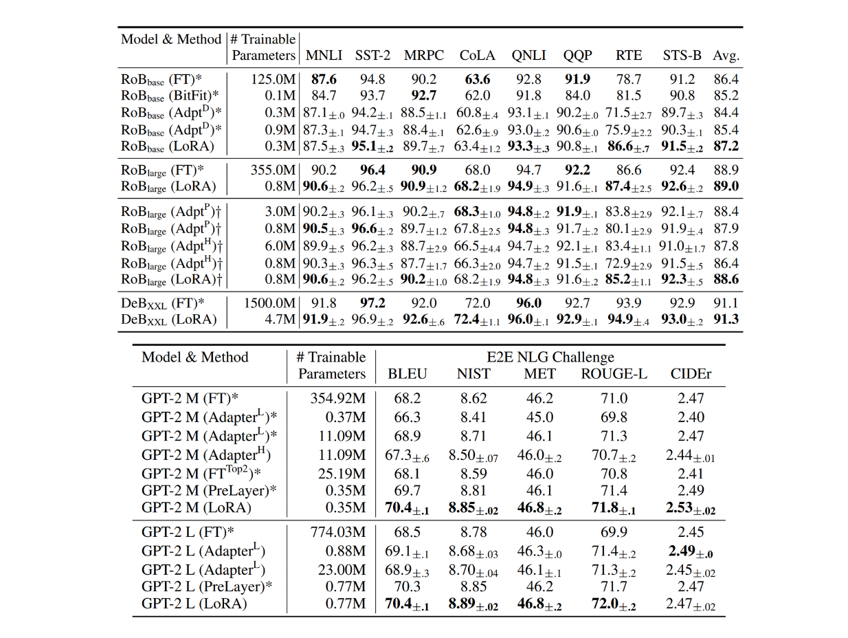Figure- RoBERTA, DEBERTA, and GPT-2 test results with different fine-tuning approaches on several benchmark datasets. .png

Figure: RoBERTA, DEBERTA, and GPT-2 test results with different fine-tuning approaches on several benchmark datasets. Source.

From the tables above, we can see that LoRA's performance is highly competitive across all tested models. The LoRA approach also outperforms other fine-tuning methods in almost all benchmark datasets. The impressive thing is that with LoRA, we can get similar or even better fine-tuned models compared to normal fine-tuning with only a fraction of trainable parameters.

To further test the capabilities of LoRA, the authors also applied this approach to the GPT-3 model, which has roughly 175B parameters, on datasets like WikiSQL and MNLI. We can see that the validation accuracy after model fine-tuning with LoRA consistently outperforms normal fine-tuning and other methods.

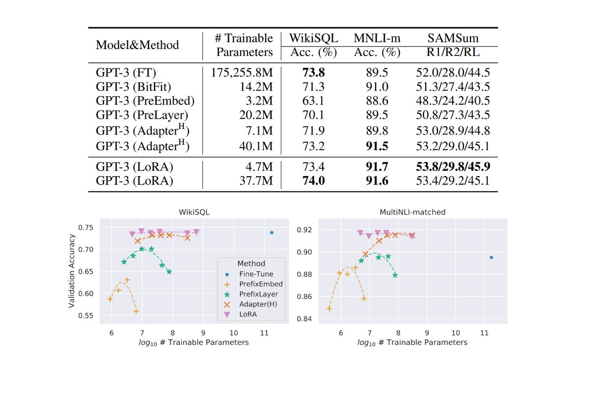Figure: GPT-3 test results with different fine-tuning approaches on WikiSQL and MNLI datasets.

Figure: l GPT-3 test results with different fine-tuning approaches on WikiSQL and MNLI datasets. Source.

Now that we know LoRA is a powerful model fine-tuning method, a question that might still arise is to which weight matrices we should apply LoRA. Given that most LLMs nowadays are based on the Transformer architecture, the authors tested the LoRA method only on the self-attention module inside each Transformer layer in a GPT-3 model.

LoRA was adapted in several weight matrices inside the self-attention module, such as in query (W_q), value (W_v), and key weights (W_k) on the same benchmark datasets mentioned above, such as WikiSQL and MNLI. You can see the experimentation results in the table below:

Figure- Validation accuracy on WikiSQL and MultiNLI after applying LoRA to different types of attention weights in GPT-3. .png

Figure: Validation accuracy on WikiSQL and MultiNLI after applying LoRA to different types of attention weights in GPT-3. Source.

It turns out that applying LoRA to both query and value weights with a rank of 4 yields the best fine-tuned model.

As mentioned previously, the rank (r) value is a hyperparameter that we need to choose in advance. The problem is, we don't know the best intrinsic rank of the weight matrices we're dealing with. To address this problem, the authors also tested LoRA with different r values. You can see the result in the table below:

Figure- Validation accuracy on WikiSQL and MultiNLI with different rank

Figure: Validation accuracy on WikiSQL and MultiNLI with different ranks. Source.

The result above shows that if we apply LoRA on both query and value weight matrices, we'll get highly competitive results even with an r value as small as 1. This suggests that the gradient weights during the fine-tuning process could have a very small intrinsic rank.

LoRA Implementation

In this section, we'll show you an example of LoRA implementation with the help of the Hugging Face library. Specifically, we'll fine-tune a BERT model on the IMDB dataset for a simple sentiment classification problem. To implement LoRA with Hugging Face, we can use the PEFT library. Let's install all the necessary libraries:

!pip install -q transformers 
!pip install -q peft
!pip install -q evaluate

Next, let's load the dataset. The IMDB dataset consists of 25,000 entries, but we'll only use a small subset for fine-tuning purposes (1,000 entries). First, we'll tokenize the entire dataset and then randomly select 1,000 entries from the tokenized data.

from datasets import load_dataset
from transformers import AutoTokenizer

def tokenize_function(examples):
    return tokenizer(examples["text"], padding="max_length", truncation=True)

dataset = load_dataset("imdb")
tokenizer = AutoTokenizer.from_pretrained("bert-base-cased")

tokenized_datasets = dataset.map(tokenize_function, batched=True)

ft_train = tokenized_datasets["train"].shuffle(seed=42).select(range(1000))
ft_val = tokenized_datasets["test"].shuffle(seed=42).select(range(1000))

Now let’s load our BERT model and set up the LoRA configuration. For the LoRA configuration, we’re going to use rank = 1 and alpha = 1. Next, we instantiate a LoRA-powered BERT using this configuration with get_peft_model method from the PEFT library.

from peft import LoraConfig, TaskType
from transformers import BertForSequenceClassification
from peft import get_peft_model

lora_config = LoraConfig(
    task_type=TaskType.SEQ_CLS, r=1, lora_alpha=1, lora_dropout=0.1
)

model = BertForSequenceClassification.from_pretrained(
    'bert-base-cased', 
    num_labels=2
)

lora_model = get_peft_model(model, lora_config)

def count_parameters(model): 

  trainable_params = sum(p.numel() for p in model.parameters() if p.requires_grad) 
  all_params = sum(p.numel() for p in model.parameters()) 
  trainable_percentage = 100 * trainable_params / all_params 
  return trainable_params, all_params, trainable_percentage 

trainable_params, all_params, trainable_percentage = count_parameters(lora_model) 

print(f"trainable params: {trainable_params} || all params: {all_params} || trainable%: {trainable_percentage}")
# Output:
trainable params: 38402 || all params: 108350212 || trainable%: 0.03544247795288116

As you can see, with LoRA, now we only need to update around 38k weights. This accounts to 0.035% of the total weights of BERT.

Finally, we can fine-tune our model. For the metrics, we’ll use the standard accuracy metrics and we’ll fine-tune it for 25 epochs. Below is the code to run the fine-tuning process.

import numpy as np
import evaluate
import wandb
from transformers import TrainingArguments, Trainer

wandb.init(mode="disabled")

def compute_metrics(eval_pred):
    logits, labels = eval_pred
    predictions = np.argmax(logits, axis=-1)
    return metric.compute(predictions=predictions, references=labels)

metric = evaluate.load("accuracy")

training_args = TrainingArguments(output_dir="test_trainer", evaluation_strategy="epoch",
                                 num_train_epochs=25,)

trainer = Trainer(
    model=lora_model,
    args=training_args,
    train_dataset=ft_train,
    eval_dataset=ft_val,
    compute_metrics=compute_metrics,
)

trainer.train()

Conclusion

LoRA provides a powerful and efficient method for fine-tuning any model, including LLMs. This method addresses the challenges of model weight storage and computation that occur with traditional fine-tuning methods. By decomposing large weight matrices into low-rank adaptations, LoRA enables us to fine-tune models for several domain-specific tasks without modifying the model's original pre-trained weights.

Compared to other fine-tuning methods like adapters, prefix tuning, and even full fine-tuning, LoRA achieved superior performance on several state-of-the-art models and benchmark datasets with only a fraction of learnable weights. As LLMs evolve, LoRA stands out as a cost-effective and scalable solution to fine-tune them.

LoRA Explained: Low-Rank Adaptation for Fine-Tuning LLMs

The Problems with Traditional Fine-Tuning Approaches

The Concept of Adapters and Prefix Tuning

The Concept of LoRA and How It Works

Experimentation Results with LoRA

LoRA Implementation

Conclusion

Further Readings

Content

Start Free, Scale Easily

Share this article