Learn
Vector Database 101: Everything You Need to Know

Introduction to Vector Similarity Search

Nov 03, 202313 min read

Learn what vector search is and the metrics pertinent to decide the distance (or similarity) between objects.

Read the entire series

In the previous tutorials, we took a look at unstructured data, vector databases, and Milvus - the world's most popular open-source vector database used for similarity search. We also briefly touched upon the idea of embeddings, high-dimensional vectors which serve as awesome semantic representations of unstructured data. One key note to remember - embeddings and vector representations which are "close" to one another represent semantically similar pieces of data.

In this introduction to vector search (aka similarity search), we'll define what it is, and answer some fundamental questions about it. Then, we will build on that knowledge by going over a word embedding example and seeing how semantically similar pieces of unstructured data are "near" one another while dissimilar pieces of unstructured data are "far" from one another. This will lead into a high-level overview of nearest neighbor search, a computing problem that involves finding the closest vector(s) to a query vector based on a unified distance metric. We'll go over some well-known methods (vector similarity search algorithms) for nearest neighbor search (including my favorite - ANNOY) in addition to commonly used distance metrics.

Let's dive in.

What is Vector Search or Vector Similarity Search?

Vector search, also known as vector similarity search or nearest neighbor search or semantic search, is a technique used in data retrieval and information retrieval systems to find items or data points that are similar or closely related to a given query vector. Unlike traditional keyword search which matches exact words or phrases, semantic search understands the intent and contextual meaning behind a query, allowing it to return more relevant results even when the exact keywords are not present in the content. In vector search, we represent data points, such as images, texts, and audio, as vectors in a high-dimensional space. The goal of vector search is to efficiently search and retrieve the most relevant vectors that are similar or nearest to a query vector.

Typically, distance metrics such as Euclidean distance or cosine similarity measure the similarity between vectors. The vector's proximity in the vector space determines how similar it is. To efficiently organize and show search results for vectors, vector search algorithms use indexing structures such as tree-based structures or hashing techniques.

Vector search is central to vector databases and has various applications, including recommendation systems, image and video retrieval, natural language processing, anomaly detection, and question and answer chatbots. Using semantic search makes it possible to find relevant items, patterns, or relationships within high-dimensional data, enabling more accurate and efficient information retrieval.

Vector search is a powerful method for analyzing and retrieving information from high-dimensional spaces. It enables users to find similar or closely related items to a given query, making it crucial in various domains. Here are the benefits of vector search:

Similarity-based Retrieval— Semantic search allows for similarity-based Retrieval, enabling users to find similar or closely related items to a given query. Similarity-based Retrieval is crucial in various domains, such as recommendation systems, where users expect personalized recommendations based on their preferences or similarities to other users.
High-dimensional Data Analysis — With the increasing availability of high-dimensional data, such as images, audio, and textual data, traditional search methods become less effective. Vector search provides a powerful way to analyze and retrieve information from high-dimensional spaces, allowing for more accurate and efficient data exploration.
Nearest-Neighbor Search — Efficient nearest-neighbor search algorithms find the nearest neighbors to a given query vector. Nearest-neighbor search is handy for critical tasks such as an image or document similarity search, content-based Retrieval, or anomaly detection that require finding the closest matches or similar items.
Improved User Experience— By leveraging semantic search, applications can provide users with more relevant and personalized results. Whether delivering relevant recommendations, retrieving visually similar images, or finding documents with similar content, vector search enhances the overall user experience by providing more targeted and meaningful results.
Scalability — Vector search algorithms and indexing structures handle large-scale datasets and high-dimensional spaces efficiently. They enable fast search and retrieval operations, making it feasible to perform similarity-based queries in real-time, even on massive datasets.

How Does a Vector Search Engine Work?

With the popularity of AI and LLMs, every developer tool, search engine, and database is adding vector search capabilities to their feature set, and due to this, the term vector engine and Vector Search Engines are often used interchangeably with Vector Databases. Vector Search Engines will conduct a Vector semantic search (sometimes referred to as Vector Search). Vector search is a technique for finding similar items or data points in a dataset based on their representation as vectors in a high-dimensional space. Each item is mapped to a point in this space, with each vector dimension representing a specific feature. The vector search process involves indexing, querying, ranking, and retrieval.

To perform vector search, you first represent your data items as vectors, using techniques like Word2Vec or for text data. An index data structure efficiently stores these vectors for quick retrieval, using methods like KD-trees or hash tables. When a user submits a query item, it's converted into a vector representation, compared to the indexed vectors using similarity metrics like cosine similarity or Euclidean distance, and the most similar items are retrieved and ranked.

Vector Search Use Cases

Image, video, audio similarity search
AI drug discovery
Semantic search engine
DNA sequence classification
Question answering system
Recommender system
Anomaly detection
Retrieval Augmented Generation (RAG)

Now that we have covered the basics of vector search, let’s look into the more technical details by looking at a word embedding example and finish with a high-level overview of nearest neighbor search.

Comparing embeddings

Once users decide they want to embark on building Vector search in their solution, the next question they often ask is “What Machine Learning Model should I use to create Vector Embeddings.” Before you can choose a model, it is important to understand vector embeddings by comparing a few examples. Let's go through a couple of word embedding examples. For the sake of simplicity, we'll use word2vec, an old model which uses a training methodology based on skipgrams. BERT and other modern transformer-based models will be able to provide you with more contextualized word embeddings, but we'll stick with word2vec for simplicity. Jay Alammar provides a great tutorial on word2vec, if you're interested in using machine learning models a bit more.

Some prep work

Before beginning, we'll need to install the gensim library and load a word2vec model.

% pip install gensim --disable-pip-version-check
% wget https://s3.amazonaws.com/dl4j-distribution/GoogleNews-vectors-negative300.bin.gz
% gunzip GoogleNews-vectors-negative300.bin

Requirement already satisfied: gensim in /Users/fzliu/.pyenv/lib/python3.8/site-packages (4.1.2)
Requirement already satisfied: smart-open>=1.8.1 in /Users/fzliu/.pyenv/lib/python3.8/site-packages (from gensim) (5.2.1)
Requirement already satisfied: numpy>=1.17.0 in /Users/fzliu/.pyenv/lib/python3.8/site-packages (from gensim) (1.19.5)
Requirement already satisfied: scipy>=0.18.1 in /Users/fzliu/.pyenv/lib/python3.8/site-packages (from gensim) (1.7.3)
--2022-02-22 00:30:34--  https://s3.amazonaws.com/dl4j-distribution/GoogleNews-vectors-negative300.bin.gz
Resolving s3.amazonaws.com (s3.amazonaws.com)... 52.216.20.165
Connecting to s3.amazonaws.com (s3.amazonaws.com)|52.216.20.165|:443... connected.
HTTP request sent, awaiting response... 200 OK
Length: 1647046227 (1.5G) [application/x-gzip]
Saving to: GoogleNews-vectors-negative300.bin.gz

GoogleNews-vectors- 100%[===================>]   1.53G  2.66MB/s    in 11m 23s

2022-02-22 00:41:57 (2.30 MB/s) - GoogleNews-vectors-negative300.bin.gz saved [1647046227/1647046227]

gunzip: GoogleNews-vectors-negative300.bin: unknown suffix -- ignored

Now that we've done all the prep work required to generate word-to-vector embeddings, let's load the trained word2vec model.

>>> from gensim.models import KeyedVectors
>>> model = KeyedVectors.load_word2vec_format('GoogleNews-vectors-negative300.bin', binary=True)

Example 0: Marlon Brando

Let's take a look at how word2vec interprets the famous actor Marlon Brando.

>>> print(model.most_similar(positive=['Marlon_Brando']))

[('Brando', 0.757453978061676), ('Humphrey_Bogart', 0.6143958568572998), ('actor_Marlon_Brando', 0.6016287207603455), ('Al_Pacino', 0.5675410032272339), ('Elia_Kazan', 0.5594002604484558), ('Steve_McQueen', 0.5539456605911255), ('Marilyn_Monroe', 0.5512186884880066), ('Jack_Nicholson', 0.5440199375152588), ('Shelley_Winters', 0.5432392954826355), ('Apocalypse_Now', 0.5306933522224426)]

Marlon Brando worked with Al Pacino in The Godfather and Elia Kazan in A Streetcar Named Desire. He also starred in Apocalypse Now.

Example 1: If all of the kings had their queens on the throne

Vectors can be added and subtracted from each other to demo underlying semantic changes.

>>> print(model.most_similar(positive=['king', 'woman'], negative=['man'], topn=1))

[('queen', 0.7118193507194519)]

Who says engineers can't enjoy a bit of dance-pop now and then?

Example 2: Apple, the company, the fruit, ... or both?

The word "apple" can refer to both the company as well as the delicious red fruit. In this example, we can see that Word2Vec retains both meanings.

>>> print(model.most_similar(positive=['samsung', 'iphone'], negative=['apple'], topn=1))
>>> print(model.most_similar(positive=['fruit'], topn=10)[9:])

[('droid_x', 0.6324754953384399)]
[('apple', 0.6410146951675415)]

"Droid" refers to Samsung's first 4G LTE smartphone ("Samsung" + "iPhone" - "Apple" = "Droid"), while "apple" is the 10th closest word to "fruit".

Vector search strategies

Now that we've seen the power of vector embeddings, let's briefly take a look at some of the ways we can conduct nearest neighbor search. This is not a comprehensive list; we'll just briefly go over some common methods in order to provide a high-level overview of how vector search is conducted at scale. Note that some of these methods are not exclusive to each other - it's possible, for example, to use quantization in conjunction with space partitioning.

(We'll also be going over each of these methods in detail in future tutorials, so stay tuned for more.)

Linear search

The simplest but most naïve nearest neighbor search algorithm is good old linear search: computing the distance from a query vector to all other vectors in the vector database.

For obvious reasons, naïve search does not work when trying to scale our vector database to tens or hundreds of millions of vectors. But when the total number of elements in the database is small, this can actually be the most efficient way to perform vector search since a separate data structure for the index is not required, while inserts and deletes can be implemented fairly easily.

Due to the lack of space complexity as well as constant space overhead associated with naïve search, this method can often outperform space partitioning even when querying across a moderate number of vectors.

Space partitioning

Space partitioning is not a single algorithm, but rather a family of algorithms that all use the same concept.

K-dimensional trees (kd-trees) are perhaps the most well-known in this family, and work by continuously bisecting the search space (splitting the vectors into “left” and “right” buckets) in a manner similar to binary search trees.

Inverted file index (IVF) is also a form of space partitioning, and works by assigning each vector to its nearest centroid - searches are then conducted by first determining the query vector's closest centroid and conducting the search around there, significantly reducing the total number of vectors that need to be searched. IVF is a fairly popular indexing strategy and is commonly combined with other indexing algorithms to improve performance.

Quantization

Quantization is a technique for reducing the total size of the database by reducing the precision of the vectors.

Scalar quantization (SQ), for example, works by multiplying high-precision floating point vectors with a scalar value, then casting the elements of the resultant vector to their nearest integers. This not only reduces the effective size of the entire database (e.g. by a factor of eight for conversion from float64_t to int8_t), but also has the positive side-effect of speeding up vector-to-vector distance computations.

Product quantization (PQ) is another quantization technique that works similar to dictionary compression. In PQ, all vectors are split into equally-sized subvectors, and each subvector is then replaced with a centroid.

Hierarchical Navigable Small Worlds (HNSW)

Hierarchical Navigable Small Worlds is a graph-based indexing and retrieval algorithm.

This works differently from product quantization: instead of improving the searchability of the database by reducing its effective size, HNSW creates a multi-layer graph from the original data. Upper layers contain only "long connections" while lower layers contain only "short connections" between vectors in the database (see the next section for an overview of vector distance metrics). Individual graph connections are created a-la skip lists.

With this architecture in place, searching becomes fairly straightforward – we greedily traverse the uppermost graph (the one with the longest inter-vector connections) for the vector closest to our query vector. We then do the same for the second layer, using the result of the first layer search as the starting point. This continues until we complete the search at the bottommost layer, the result of which becomes the nearest neighbor of the query vector.

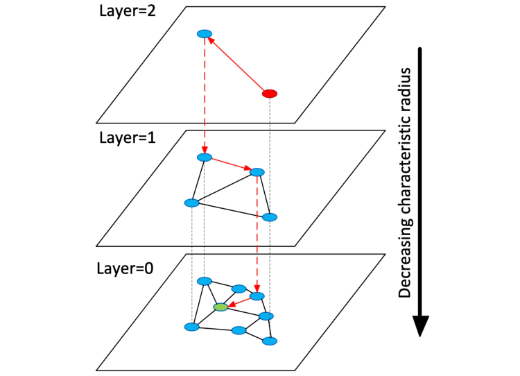HNSW, visualized. Image source: https://arxiv.org/abs/1603.09320

Approximate Nearest Neighbors Oh Yeah

This is probably my favorite ANN algorithm simply due to its playful and unintunitive name. Approximate Nearest Neighbors Oh Yeah (ANNOY) is a tree-based algorithm popularized by Spotify (it’s used in their music recommendation system). Despite the strange name, the underlying concept behind ANNOY is actually fairly simple – binary trees.

ANNOY works by first randomly selecting two vectors in the database and bisecting the search space along the hyperplane separating those two vectors. This is done iteratively until there are fewer than some predefined parameter NUM_MAX_ELEMS per node. Since the resulting index is essentially a binary tree, this allows us to do our search on O(log n) complexity.

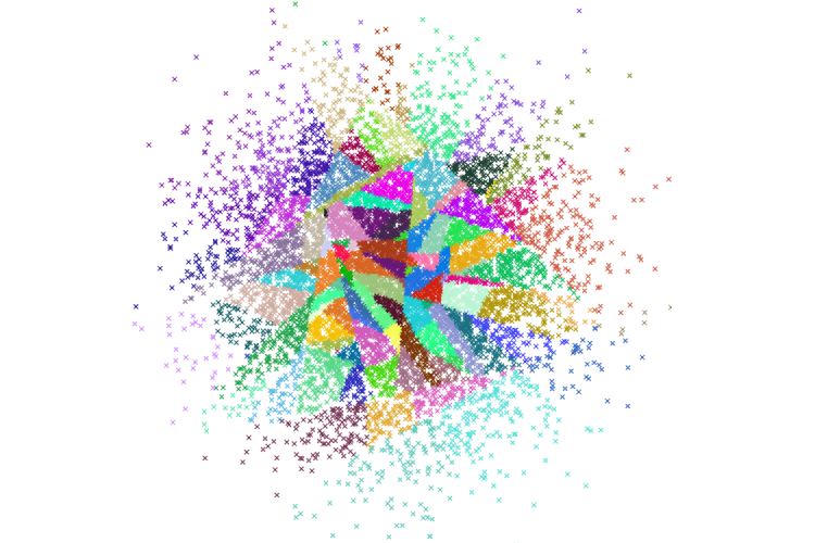ANNOY, visualized. Image source: https://github.com/spotify/annoy

Commonly used similarity metrics

The very best vector databases are useless without similarity metrics – methods for computing the distance between two vectors. Numerous metrics exist, so we will discuss only the most commonly used subset here.

Floating point vector similarity metrics

The most common floating point vector similarity metrics are, in no particular order, L1 distance, L2 distance, and cosine similarity. The first two values are distance metrics (lower values imply more similarity while higher values imply lower similarity), while cosine similarity is a similarity metric (higher values imply more simlarity).

$d_{l1}(\mathbf{a},\mathbf{b})=\sum_{i=1}^{N}|\mathbf{a}_i-\mathbf{b}_i|$
$d_{l2}(\mathbf{a},\mathbf{b})=\sqrt{\sum_{i=1}^{N}(\mathbf{a}_i-\mathbf{b}_i)^2}$
$d_{cos}(\mathbf{a},\mathbf{b})=\frac{\mathbf{a}\cdot\mathbf{b}}{|\mathbf{a}||\mathbf{b}|}$

L1 distance is also commonly referred to as Manhattan distance, aptly named after the fact that getting from point A to point B in Manhattan requires moving along one of two perpendicular directions. The second equation, L2 distance, is simply the distance between two vectors in Euclidean space. The third and final equation is cosine distance, equivalent to the cosine of the angle between two vectors. Note the equation for cosine similarity works out to be the dot product between normalized versions of input vectors a and b.

With a bit of math, we can also show that L2 distance and cosine similarity are effectively equivalent when it comes to similarity ranking for unit norm vectors:

$d_{l2}(\mathbf{a},\mathbf{b})=(\mathbf{a}-\mathbf{b})^T(\mathbf{a}-\mathbf{b})$ $=\mathbf{a}^T\mathbf{a}-2\mathbf{a}^T\mathbf{b}+\mathbf{b}^T\mathbf{b}$

Recall that unit norm vectors have a magnitude of 1:

$\mathbf{a}^T\mathbf{a}=1$

With this, we get:

$\mathbf{a}^T\mathbf{a}-2\mathbf{a}^T\mathbf{b}+\mathbf{b}^T\mathbf{b}$ $=2-2\mathbf{a}^T\mathbf{b}$

Since we have unit norm vectors, cosine distance works out to be the dot product between a and b (the denominator in equation 3 above works out to be 1):

$2-2\mathbf{a}^T\mathbf{b}$ $=2(1-d_{cos}(\mathbf{a},\mathbf{b}))$

Essentially, for unit norm vectors, L2 distance and cosine similarity are functionally equivalent! Always remember to normalize your embeddings.

Binary vector similarity metrics

Binary vectors, as their name suggest, do not have metrics based in arithmetics a-la floating point vectors. Similarity metrics for binary vectors instead rely on either set mathematics, bit manipulation, or a combination of both (it's okay, I also hate discrete math). Here are the formulas for two commonly used binary vector similarity metrics:

$d_J(\mathbf{a},\mathbf{b})=1-\frac{\mathbf{a}\cdot\mathbf{b}}{|a|^2+|b|^2-\mathbf{a}\cdot\mathbf{b}}$
$d_J(\mathbf{a},\mathbf{b})=\sum_{i=1}^{N}\mathbf{a}_i\oplus\mathbf{b}_i$

The first equation is called Tanimoto/Jaccard distance, and is essentially a measure of the amount of overlap between two binary vectors. The second equation is Hamming distance, and is a count of the number of vector elements in a and b which differ from each other.

You can most likely safely ignore these similarity metrics, since the majority of applications use cosine similarity over floating point embeddings.

Wrapping up

In this tutorial, we took a look at vector search, along with some common vector search algorithms and distance metrics. Here are some key takeaways:

Embedding vectors are powerful representations, both in terms of distance between the vectors and in terms of vector arithmetic. By applying a liberal quantity of vector algebra to embeddings, we can perform scalable semantic analysis using just basic mathematical operators.
Semantic Vector search overcomes the limitation of keyword search by enabling you to search based on the meaning of your query. It enables quick retrieval of answers by performing vector search.
There are a wide variety of approximate nearest neighbor search algorithms and/or index types to choose from. The most commonly one used today is HNSW, but a different indexing algorithm may work better for your particular application, depending on the total number of vector embeddings you have in addition to the length of each individual vector.
The two primary distance metrics used today are L2/Euclidean distance and cosine distance. These two metrics, when used on normalized embeddings, are functionally equivalent.

Thanks for joining us for this tutorial! Vector search is a core part of Milvus, and it will continue to be. In future tutorials, we'll be doing some deeper dives into the most commonly used ANNS algorithms - HNSW and ScaNN.

Take another look at the Vector Database 101 courses

Updated on Mar 27, 2025

Zilliz

Next: Everything You Need to Know about Vector Index Basics

Content

Start Free, Scale Easily

Try the fully-managed vector database built for your GenAI applications.

Try Zilliz Cloud for Free

Share this article

Keep Reading

Introduction to Unstructured Data

Buckle up for the first tutorial in our Vector Database 101 series and untangle the intricacy around Milvus with us every week.

Understanding Vector Databases: Compare Vector Databases, Vector Search Libraries, and Vector Search Plugins

Deep diving into better understanding vector databases and comparing them to vector search libraries and vector search plugins.

Integrating Vector Databases with Cloud Computing: A Strategic Solution to Modern Data Challenges

Integrating vector databases and cloud computing creates a powerful infrastructure that significantly enhances the management of large-scale, complex data in AI and machine learning.