Learn
Natural Language Processing (NLP) Advanced Guide

Primer on Neural Networks and Embeddings for Language Models

Nov 14, 20239 min read

Exploring neural network language models, specifically recurrent neural networks, and taking a sneak peek at how embeddings are generated.

By Frank Liu

Read the entire series

Introduction

In the previous post, we covered the basics of natural language processing - tokens in natural language and n-gram and bag-of-words language models. While these models are simple to understand, they are an undoubtedly weak baseline. In this post, we'll dive into neural network language models, specifically recurrent neural networks, and take a sneak peek at how embeddings are generated. Let's dive in.

Anatomy of a neural network

We'll first briefly review the anatomy of a neural network, i.e., neurons, multilayer networks, and backpropagation. Please note that this is not a crash course but a summary for those familiar with deep learning. There are many great and much more detailed resources out there (e.g., CS231n course notes).

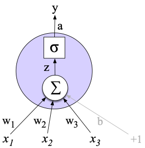
In machine learning, a neuron is a single unit that forms the basis for all neural networks. At its core, a neuron is a single unit within a neural network that takes a weighted sum of all its inputs and adds an optional bias term. In the form of an equation, it looks like this:

$q = \sum_{i=0}^{n-1}w_ix_i + b q = \mathbf{w}\mathbf{x} + b$

Here, $x_0$ , $x_1$ , ..., $x_{n-1}$ represent the outputs from the previous layer of neurons, and $w_0$ , $w_1$ , ..., $w_{n-1}$ represent the weights that this neuron uses to synthesize the output value.

If a multi-layer neural network were composed of only the weighted sums in the equation above, we could collapse all terms into a single linear layer - not exactly ideal for understanding the relationship between tokens or encoding complex text. All neurons include a non-linear activation function after the weighted sum. The Rectified Linear Unit (ReLU) function is a well-known example:

$ReLU(q) = \begin{array}{cc} \Bigg\{ & \begin{array}{cc} 0 & q\leq 0 \\ q & q\geq q \end{array} \end{array}$

For most modern neural network language models, the Gaussian Error Linear Unit* (GELU) activation is much more popular:

$\begin{array}{cc} GELU(q) &= q\Phi{q} \end{array}$

Here, $\Phi{q}$ represents the Gaussian cumulative distribution function, and can be approximated with $GELU(q) \approx \frac{q}{1 + e^{-1.702q}}$ . This activation gets applied after the weighted sum described above. All-in-all, a single neuron looks something like this:

A visualization of a single neuron (weights and activation function)

To learn more complex functions, we can stack neurons - one on top of another - to form a layer. All neurons in a layer receive the same input as others in the same layer; the only difference between them is the weights $\mathbf{w}$ and biases $b$ . We can now express the equation above in matrix notation to denote a single layer.

$\mathbf{y} = GELU(\mathbf{W}\mathbf{x} + \mathbf{b})$

Here, $\mathbf{W}$ is a two-dimensional matrix that contains all weights applied to the inputs $\mathbf{x}$ ; each row of the matrix corresponds to the weights of a single neuron. This type of layer is often called a dense layer or fully connected layer since all inputs $\mathbf{x}$ are connected to all outputs $\mathbf{y}$ .

We can chain two of these layers together to create a basic feedforward network:

A standard feedforward network. The arrows between each blue circle are the output values of each neuron (the "activations").

Image source: Source

Note how we've introduced a new hidden layer $\mathbf{h_1}$ with no direct connection to the input $\mathbf{x}$ nor output $\mathbf{y}$ . This layer has effectively allowed us to add extra depth to the network, consequently increasing the total number of parameters (there are now multiple weight matrices $\mathbf{W}$ ) and its representative power. One important thing to note as more hidden layers are added: hidden values (activations) from layers closer to the input are more "similar" to $\mathbf{x}$ , while activations closer to the output are more similar to $\mathbf{y}$ . Please keep this in mind as we move forward - hidden layers are extremely important for understanding vector search, which we'll continue to return to as we experiment with vector embeddings in future posts.

Parameters for an individual neuron in a feedforward network can be updated through a process called backpropagation, which is a repeated application of the chain rule in calculus. Whole courses are taught on backpropogation and why it seems to work so well for training neural networks, so that we won't cover the a to z of backpropagation here, but the basic process looks like this:

Feed a batch of input data through the neural network.
Calculate the loss. This is usually the L2 loss (squared difference) for regression and cross-entropy loss for classification.
Use this loss to compute the gradients of the loss with respect to weights in the final hidden layer $\frac{\partial{\Lambda}}{\partial{\W_n}}$ .
Compute the loss through the final hidden layer, i.e. $\frac{\partial{\Lambda}}{\partial{\h_{n-1}}}$ .
Backpropogate this loss to the weights of the second-to-last hidden layer $\frac{\partial{\Lambda}}{\partial{\W_{n-1}}}$ .
Repeat steps 4 and 5 until partial derivatives for all weights are computed.

With partial derivatives of the loss with respect to all weights in the network, a single large weight update can then be performed according to the optimizer and learning rate. This is done repeatedly until either 1) the model converges or 2) all epochs are finished.

Recurrent neural networks

All forms of text and natural language are inherently sequential, meaning that words/tokens are processed one after another, and seeming simple changes such as the addition of a single token, the reversal of two consecutive tokens, or the addition of punctuation can potentially result in enormous differences in interpretation. For example, the phrases "let's eat, Charles" and "let's eat Charles" mean two completely different things, while the phrases "we're here to help" and "we're here to help" have almost identical meanings. Combined with the sequential nature of natural language, this property makes neural networks with recurrence, i.e. recurrent neural networks (RNNs), a natural choice for language modeling.

For those unfamiliar with RNNs, recurrence is a special form of recursion where the function is a neural network rather than code. RNNs also have a natural biological origin - the human brain is analogous to an (artificial) neural network, and the words we type or speak result from biological processing.

An RNN has two components: 1) a standard feedforward network and 2) a recursive component. The feedforward network is the same as we've covered in the previous section. For the recursive component, the final hidden state is fed back into the input so that the network can maintain the prior context. As such, at each and every new timestep, prior knowledge (in the form of the previous timestep's hidden layer) is injected into the network.

An RNN, visualized. "a" denotes the hidden states, while "x" and "y" denote the inputs and outputs, respectively

Image source

Given this high-level definition of an RNN, we can envision how it is implemented and why it might work well. First, this cyclical structure of RNNs allows them to capture and process data sequentially, similar to how humans speak, read, and write. Furthermore, RNNs also effectively have access to "information" from previous time steps, making them better than n-gram models and pure feedforward networks for understanding natural language.

Let's implement one together using PyTorch. Note that this will require a solid understanding of PyTorch fundamentals; the PyTorch 60-minute blitz is a great place to start if you don't feel comfortable.

We'll first define a simple feedforward network, then expand into a simple RNN. Let's define the layers first:

from torch import Tensor
import torch.nn as nn

class BasicNN(nn.Module):
    def __init__(self, in_dims: int, hidden_dims: int, out_dims: int):
        super(BasicNN, self).__init__()
        self.w0 = nn.Linear(in_dims, hidden_dims)
        self.w1 = nn.Linear(hidden_dims, out_dims)

Note that we have not yet defined what the loss will look like as we're merely outputting the raw logits - when training, you'll want to tack on some sort of criterion such as nn.CrossEntropyLoss.

With this complete, we can implement the forward pass:

    def forward(self, x: Tensor):
        h = self.w0(x)
        y = self.w1(h)
        return y

These two code snippets combine to form a basic feedforward neural network. To make it an RNN, we have to add a feedback loop from the final hidden state back to the input:

    def forward(self, x: Tensor, h_p: Tensor):
        h = self.w0(torch.cat(x, h_p))
        y = self.w1(h)
        return (y, h)

And that's pretty much it is that simple. Since we have now increased the number of inputs to the layer of neurons defined by w0, we'll need to update its definition in __init__ as well. Let's do that and put it all together into a single code snippet:

import torch.nn as nn
from torch import Tensor

class SimpleRNN(nn.Module):
    def __init__(self, in_dims: int, hidden_dims: int, out_dims: int):
        super(RNN, self).__init__()
        self.w0 = nn.Linear(in_dims + hidden_dims, hidden_dims)
        self.w1 = nn.Linear(hidden_dims, out_dims)

    def forward(self, x: Tensor, h_p: Tensor):
        h = self.w0(torch.cat(x, h_p))
        y = self.w1(h)
        return (y, h)

The activations from the hidden layer h are returned along with the output at every forward pass. These activations can then be passed back into the model along with every new token in the sequence. The pseudocode for such a process looks like this:

model = SimpleRNN(n_in, n_hidden, n_out)

...

h = torch.zeros(1, n_hidden)
for token in range(seq):
    (out, h) = model(token, )

That's it for our implementation!

Language model embeddings

The hidden layer in the example we saw above effectively encodes everything (all tokens) that has been input into the RNN already. More specifically, all information necessary to parse the text the RNN has seen should be contained within the activations $\mathbf{h}$ . Another way of saying this is that $\mathbf{h}$ encodes the semantics of the input sequence, and the collective ordered floating point values defined by $\mathbf{h}$ can be more aptly called an embedding vector, or an embedding for short.

These representations are extremely powerful and broadly form the basis for vector search and databases. Although today's embeddings for natural language are generated from another class of machine learning models called transformers rather than RNNs, the idea remains the exact same: embeddings encode everything a computer needs to know about the content of the text. We'll go over exactly how these vectors can be used in the next blog post.

Wrapping up

In this post, we implemented a very simple recurrent neural network in PyTorch and briefly discussed language model embeddings. While recurrent neural networks are a powerful tool for understanding language and can be applied broadly across various applications (machine translation, classification, question-answering, etc), they are still not the type of ML model used to generate embeddings.

In the next tutorial, we'll use open-source transformer models to generate embeddings and perform vector search and arithmetic across them to show how powerful these learned representations truly are. We'll also circle back to the idea of bag-of-words models to see how the two may be used together to encode lexical and semantic meaning. Stay tuned!

Frank Liu
Frank Liu is the Director of Operations & ML Architect at Zilliz, where he serves as a maintainer for the Towhee open-source project. Prior to Zilliz, Frank co-founded Orion Innovations, an ML-powered indoor positioning startup based in Shanghai and worked as an ML engineer at Yahoo in San Francisco. In his free time, Frank enjoys playing chess, swimming, and powerlifting. Frank holds MS and BS degrees in Electrical Engineering from Stanford University.

Next: Sparse and Dense Embeddings

Content

Start Free, Scale Easily

Try the fully-managed vector database built for your GenAI applications.

Try Zilliz Cloud for Free