Learn
Class Activation Mapping (CAM): Better Interpretability in Deep Learning Models

Class Activation Mapping (CAM): Better Interpretability in Deep Learning Models

Mar 25, 202411 min read

Class Activation Mapping (CAM) is used to visualize and understand the decision-making of convolutional neural networks (CNNs) for computer vision tasks.

By Ruben Winastwan

Read the entire series

What is the importance of the Class Activation Mapping method?

Deep learning models often outperform traditional machine learning methods in complex tasks. However, they come with a significant limitation: interpretability.

Deep learning models' predictions are notoriously difficult to interpret. This lack of transparency makes it challenging to understand the reasons behind the model's decisions, thus reducing its trustworthiness. Researchers have proposed several methods to address this issue, including Class Activation Mapping (CAM), which is a powerful technique for visualizing and understanding the decision-making process of convolutional neural networks (CNNs) for computer vision tasks.

In this article, we will explore the importance of Class Activation Mapping in CNNs, learn the theory behind CAM, and learn how to implement it in code. So, without further ado, let's get started!

Why Do We Need Class Activation Mapping (CAM)?

Convolutional neural networks (CNNs) are commonly applied to solve various computer vision tasks, including image classification, image segmentation, object detection, object localization, and pose estimation.

How convolutional neural network models detect items in images

However, deep learning networks, including CNNs, are often perceived as black boxes. We feed them input data, and they produce predictions based on the tasks they’ve been trained for. Understanding their decision-making process can be incredibly challenging because CNNs typically consist of multiple layers with complex interactions.

On the other hand, interpretability is very crucial in all machine learning models to ensure its trustworthiness. In the context of CNNs, it’s important to verify that the model focuses on the correct regions of an image when making predictions.

Let’s say that we develop an autonomous vehicle system. Suppose we build an image classification model to identify objects on the street. The vehicle will then act based on the objects predicted by the model. In such situations, it’s important to ensure that the model correctly identifies the relevant regions of the image when making predictions; otherwise, the vehicle may malfunction.

Class Activation Mapping is an early method designed to address this problem. It allows us to investigate the regions of an image that influence the model’s predictions.

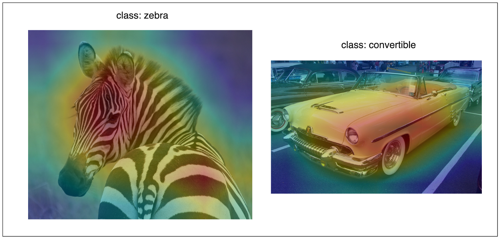Heatmap: A Class Activation Map highlights the regions around the zebra and car as more significant than other image parts.

As shown in the heatmap above, implementing a Class Activation Map highlights the regions around the zebra and car as more significant than other image parts. The heatmap’s intensity corresponds to the region’s importance for the model’s prediction. Therefore, this method improves the transparency and trustworthiness of the model.

What is Class Activation Mapping (CAM)?

Before diving into how Class Activation Mapping works, let's review the typical architecture of CNN-based models. CNN-based models consist of multiple convolutional layers, as shown in the image below. As the input image passes through each convolutional layer, its dimensions decrease while the number of features increases.

How a CNN model works

After passing through the last convolutional layer, the values within each feature map are aggregated using the Global Average Pooling Layer (GAP). Following the GAP layer, each feature map is represented by a single scalar value. Next, these values are fed into a final feed-forward layer to produce the model's prediction.

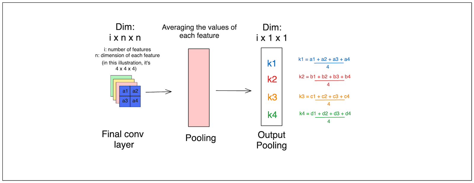How the last convolutional layer works

So, how do we derive the Class Activation Maps from this process?

The predictions of CNN-based models are generated within the final feed-forward layer. Within this layer, the value of each feature map is multiplied by its weight for a specific class and then summed to yield the final value for that class. Here's the intuition behind the weight of each feature:

If the weight > 0, the corresponding feature increases the likelihood that our input image belongs to a particular class.
If the weight = 0, the corresponding feature has no impact.
If the weight < 0, the corresponding feature decreases the likelihood that our input image belongs to a particular class.

Consequently, our model's prediction corresponds to the class with the highest weighted sum of the features.

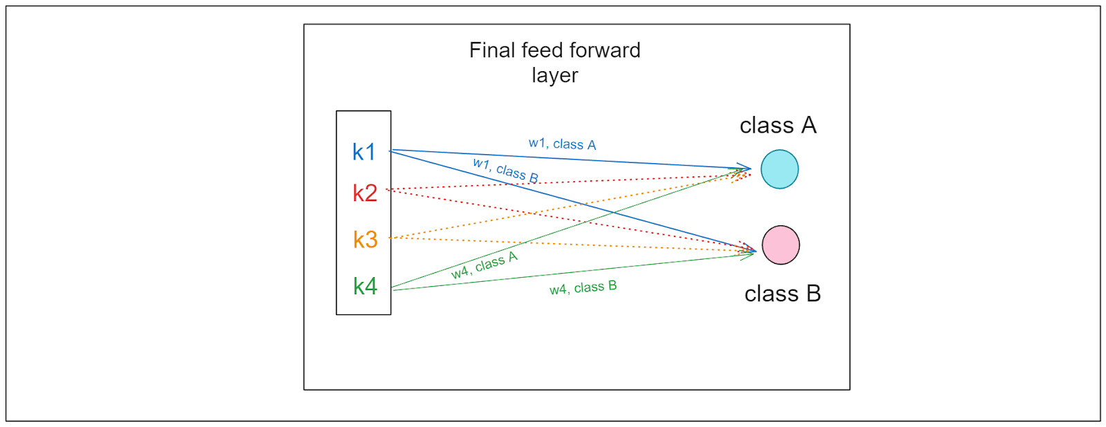How the feed forward layer works

Here is the idea: if we can obtain the weight of each feature map for our predicted class, we can assess its importance in the convolutional neural network model's prediction!

Once we obtain the weight of each feature map for the predicted class, the next steps are straightforward. First, we must fetch the feature maps from the final convolutional layer (prior to the global average pooling layer). Second, we multiply each feature map by its corresponding weight. Finally, we sum these multiplication results to obtain a single matrix with dimensions matching those of the feature maps in the final convolutional layer.

Let's use the illustrations above to clarify. Suppose our model predicts that the input image belongs to class A. Our goal is to identify the regions of the image that influenced this prediction.

To compute the CAM:

We retrieve the weight of each feature map for class A, denoted as (w1, class A), (w2, class A), (w3, class A), and (w4, class A).
We also need to obtain the feature maps from the last convolutional layer (in the illustration above, this corresponds to the feature with dimensions of 4 x 4 x 4).

Finally, we calculate the weighted sum for each feature map, resulting in a matrix as shown below:

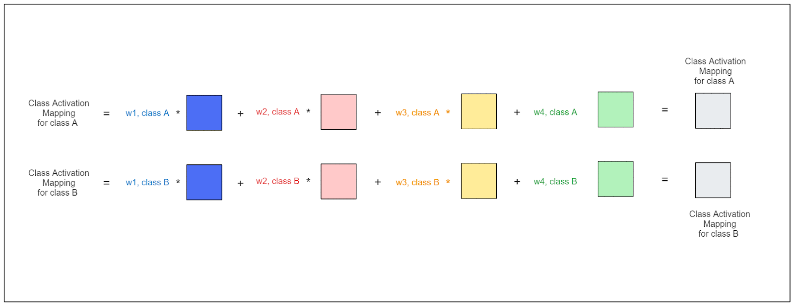Calculating the weighted sum for each feature map

The regions in the matrix with high values are crucial for the model's prediction. The last step involves upscaling this matrix to the original dimensions of our input image. In the visualization, the regions with high values will be more prominent, as shown in the previous section.

Class Activation Mapping Implementation

In this section, we will implement CAM from scratch using PyTorch. It means that we won’t rely on any high-level libraries that abstract the entire process of generating CAM. You can, of course, use TensorFlow instead. However, you need to adjust several things in the following tutorial according to their API if you wish to do so.

First, let's import all the necessary libraries for the implementation.

import numpy as np
import cv2
from torchvision import models, transforms
from torch.nn import functional as F

The numpy library is used for computing the weighted sum of the feature maps to obtain the final CAM. Meanwhile, OpenCV will be used for image preprocessing, and torchvision is a library where we can access common pretrained models for computer vision tasks.

The model we're using for this implementation is ResNet18. As the name suggests, it consists of 18 convolutional layers and has been trained on over a million images from the ImageNet database, which includes 1,000 distinct classes. Let's now load the pre-trained model.

model = models.resnet18(pretrained=True)
model = model.eval()

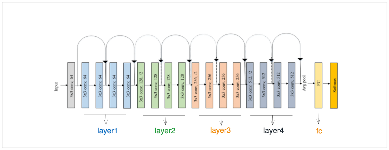How ResNet18 works

As you can see from the illustration above, the 18 convolutional layers of ResNet18 are divided into four blocks before the GAP layer and the final feed-forward layer. As you already know from the previous section, we need to store the feature maps from the final convolutional layer before the GAP layer in order to calculate CAM.

The feature maps that we want to store are essentially the output of the fourth block, named 'layer4'. One approach to store the output of 'layer4' is by using the register_forward_hook method from PyTorch. This method will store intermediate results from a particular layer during the forward pass.

# define a function to store the feature maps at the final convolutional layer
activation = {}
def getActivation(name):
    # the hook signature
    def hook(model, input, output):
        activation[name] = output.detach()
    return hook

model.layer4.register_forward_hook(getActivation('final_conv'))

Next, let’s load our input image by providing the path to our image.

# you can use any image, for this example, we'll use an image of a dog
image_path = "path_to_your_image.png"

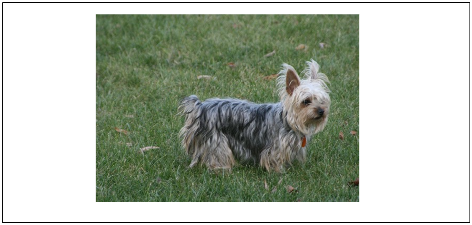The image of a dog

We’ll use an image of a silky terrier dog for this example. Our goal is to find out the model's prediction for this image and identify the regions within the image that influence the model's prediction.

One important thing to note is that ResNet18 has been pre-trained on images with dimensions of 224 x 224, along with specific mean and standard deviation values. Therefore, we need to transform our image by resizing it first and then normalizing it according to the mean and standard deviation of the ImageNet dataset.

Additionally, when we load our image using OpenCV, the default channel of our image is in BGR format. Thus, we need to convert it to RGB as well.

# define the data transformation pipeline: resize => tensor => normalize
transforms = transforms.Compose(
    [transforms.ToPILImage(),
     transforms.Resize((224, 224)),
     transforms.ToTensor(),
     transforms.Normalize(
        mean=[0.485, 0.456, 0.406],
        std=[0.229, 0.224, 0.225]
    )
    ]
)

image = cv2.imread(image_path)
orig_image = image.copy()

image = cv2.cvtColor(image, cv2.COLOR_BGR2RGB)
height, width, _ = image.shape

Now let’s do the forward pass on our input image using our ResNet18 model. At the end, we fetch the index of the predicted class.

# apply the image transforms
image_tensor = transforms(image)
# add batch dimension
image_tensor = image_tensor.unsqueeze(0)
# forward pass through model
outputs = model(image_tensor)
# get the idx of predicted class
class_idx = F.softmax(outputs).argmax().item()
print(class_idx) # output: 201

If you refer to the label mapping of the ImageNet data, which you can find here, you'll see that index 201 corresponds to a silky terrier. This means that the model’s prediction is correct. The role of CAM is to highlight the regions in the image that are crucial for the model to predict it as a silky terrier.

As mentioned in the previous section, to calculate the CAM, we need to retrieve two things:

The feature maps from the final convolutional layer.
The weight of each feature map learned from the final feed-forward layer.

Fetching the feature maps from the final convolutional layer is straightforward, as we've already implemented the register_forward_hook before. Similarly, obtaining the weight of each feature from the final feed-forward layer is also simple. All we need to do is specify the name of the corresponding feed-forward layer, which in ResNet18 is referred to as 'fc'.

# Fetch feature maps at the final convolutional layer
conv_features = activation['final_conv']

# Fetch the learned weights at the final feed-forward layer
weight_fc = model.fc.weight.detach().numpy()

Now, it's time to compute the CAM. To obtain the CAM, we need to calculate the weighted sum of the feature maps, which is essentially a dot product between the weights and the feature maps.

Afterwards, we need to denormalize the CAM and upsample it to match the dimensions of the input image. By doing so, we can overlay the CAM result on top of the original image to generate the heatmap visualization.

def calculate_cam(feature_conv, weight_fc, class_idx):
    
    # generate the class activation maps upsample to 224x224
    size_upsample = (224, 224)
  
    bz, nc, h, w = feature_conv.shape

    cam = weight_fc[class_idx].dot(feature_conv.reshape((nc, h*w)))
    cam = cam.reshape(h, w)
    cam = cam - np.min(cam)
    cam_img = cam / np.max(cam)
    cam_img = np.uint8(255 * cam_img)
    output_cam = cv2.resize(cam_img, size_upsample)

    return output_cam

# generate class activation mapping
class_activation_map = calculate_cam(conv_features, weight_fc, class_idx)

Finally, let’s create a function for model visualization, i.e, the overlay between CAM and the original input image, with the following method:

def visualize_cam(class_activation_map, width, height, orig_image):

    heatmap = cv2.applyColorMap(cv2.resize(class_activation_map,(width, height)), cv2.COLORMAP_JET)
    result = heatmap * 0.3 + orig_image * 0.5
    
    cv2.imshow(result)
    cv2.waitKey(0)
 
# visualize result
visualize_cam(class_activation_map, width, height, orig_image)

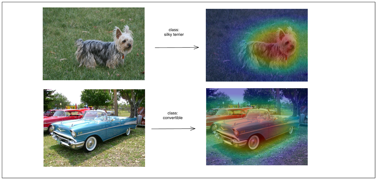Visualize the result of CAM

Improvement of Class Activation Mapping (CAM)

Class Activation Mapping is an early method that initiated the rapid development in AI interpretability, particularly for computer vision tasks. Currently, many methods based on CAM have been proposed to improve its accuracy and flexibility, such as GradCAM and GradCAM++.

As you may already know, to use Class Activation Mapping, we need to use models with a specific architecture. Specifically, we need to aggregate feature maps from the last convolutional layer using a GAP (Global Average Pooling) layer. If our model doesn't have a GAP layer at the end, implementing CAM would require modifying the model's architecture.

GradCAM generalizes this approach, eliminating the need for a GAP layer in the model, allowing us to use any CNN-based architecture to generate Class Activation Maps.

More recently, a method called GradCAM++ was proposed as an enhancement to GradCAM. This method provides better visual explanations of the model's predictions, especially in cases where multiple objects influence the prediction within a single image.

If you would like to learn more about GradCAM or GradCAM++, we recommend referring to their official research papers.

Concluding thoughts on Class Activation Maps

In this article, we've covered everything you need to know about Class Activation Mapping. First, we discussed the importance of being able to interpret the predictions of our deep learning model and how Class Activation Maps can assist us in this regard. Then, we learned about the underlying process of CAM to generate heat maps, visualizing the regions that significantly influence the model's prediction. Finally, we implemented CAM from scratch without relying on any high-level libraries to ensure a comprehensive understanding of the CAM generation process.

We hope that this article is useful for you to get started with Class Activation Mapping, or explainable AI in general. CAM is a straightforward method to interpret the prediction of convolutional neural network-based models, making it a perfect entry point if you’re just getting started in explainable AI.

Class Activation Mapping (CAM): Better Interpretability in Deep Learning Models

What is the importance of the Class Activation Mapping method?

Why Do We Need Class Activation Mapping (CAM)?

What is Class Activation Mapping (CAM)?

Class Activation Mapping Implementation

Improvement of Class Activation Mapping (CAM)

Concluding thoughts on Class Activation Maps

Further Reading

Content

Start Free, Scale Easily

Share this article