Blog
Best Practices in Implementing Retrieval-Augmented Generation (RAG) Applications

Best Practices in Implementing Retrieval-Augmented Generation (RAG) Applications

Oct 21, 202416 min read

Retrieval-Augmented Generation (RAG) is a method that has proven very effective in improving LLMs' responses and addressing LLM hallucinations. In a nutshell, RAG provides LLMs with context that can help them generate more accurate and contextualized responses. The contexts can come from anywhere: from your internal documents, vector databases, CSV files, JSON files, etc.

RAG is a novel approach that consists of many components that work together. These components include query processing, context chunking, context retrieval, context reranking, and the LLM itself to generate the response. Each component influences the quality of the final response generated from a RAG application. The problem is that it's difficult to find the best combination of methods in each component that leads to the most optimal RAG performance.

In this article, we will discuss several techniques commonly used in all RAG components, evaluate the best approach for each component, and then find the best combination that leads to the most optimal RAG-generated response, according to this paper. So, without further ado, let's start with an introduction to RAG components.

RAG Components

As mentioned, RAG is a powerful method to alleviate LLMs' hallucination problems, which commonly occur when we ask queries beyond their training data or when they require specialized knowledge. For example, if we ask an LLM a question about our internal data, we will likely get an inaccurate answer. RAG solves this problem by providing our LLM with context that can help answer our query.

RAG consists of a chain of components that form a workflow. The typical RAG components include:

Query classification: to determine whether our query needs retrieval of contexts or can be processed directly by the LLM.
Context retrieval: to fetch the top k candidates in the most relevant contexts to our query.
Context reranking: to sort the top k candidates fetched from the retrieval component, starting with the most similar one.
Context repacking: to organize the most relevant contexts into a more structured format for better response generation.
Context summarization: to extract key information from relevant contexts for improved response generation.
Response generation: to generate a response based on the query and relevant contexts.

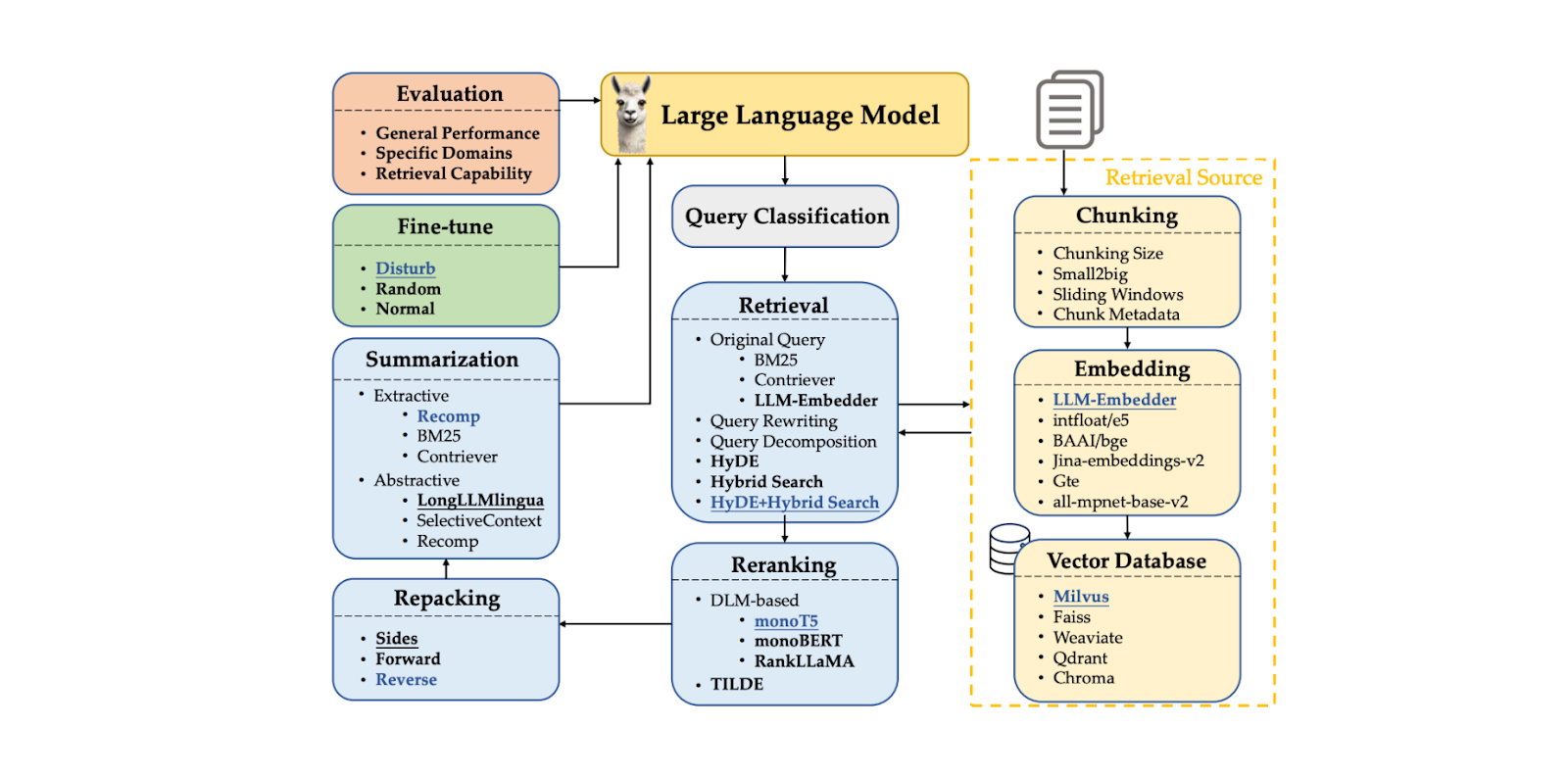Figure- RAG Components..png

Figure: RAG Components. Source

While these RAG components are useful during the response generation process (i.e., when we've already stored all contexts and they're ready to be fetched), several other factors must be considered before implementing a RAG method.

We need to transform our context documents into vector embeddings to make our context documents useful in a RAG approach. Therefore, choosing the most appropriate embedding model and strategy to represent our input documents as embeddings is crucial.

An embedding contains a semantically rich representation of our input document. However, if the document used as context is too long, it can confuse the LLM when generating an appropriate response. A common approach to solving this problem is to apply a chunking method, where we split our input document into several chunks and then transform each chunk into an embedding. It's crucial to pick the best chunking method and size, as chunks that are too short will likely contain insufficient information.

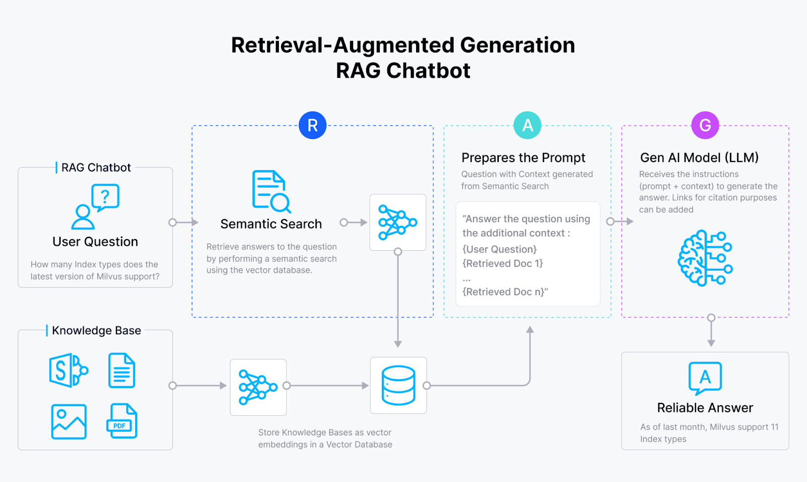Figure- RAG workflow.png

Figure: RAG workflow

We must consider appropriate storage for these embeddings once we transform each chunk into an embedding. If you're not dealing with many embeddings, you can store them directly in your device's local memory. However, you'll commonly deal with hundreds or even millions of embeddings in practice. In this case, you need a vector database like Milvus or its managed service, Zilliz Cloud, to store them, and choosing the right vector database is crucial for the success of our RAG application.

The final consideration is the LLM itself. If applicable, we can fine-tune the LLM to target our specific needs more precisely. However, fine-tuning is costly and unnecessary in most cases, especially if we're using a performant LLM with many parameters.

In the following sections, we'll discuss the best approaches for each RAG component. Next, we'll explore combinations of these best approaches and suggest several strategies for deploying RAG that balance performance and efficiency.

Query Classification

As mentioned in the previous section, RAG is useful in ensuring that the LLM generates accurate and contextualized responses, especially when specialized knowledge from our internal data is required. However, RAG also increases the runtime of the response generation process. The thing is, not all queries require the retrieval process, and many of them can be processed directly by the LLM. Therefore, skipping the context retrieval process would be more beneficial if a query doesn't need it.

We can implement a query classification model to determine whether a query needs context retrieval before the response generation process. Such a classification model usually consists of a supervised model, such as BERT, with the main goal of predicting whether a query needs retrieval or not. However, like other supervised models, we must train it before using it for inference. To train the model, we need to generate a dataset of example prompts and their corresponding binary labels, including whether the prompt needs retrieval or not.

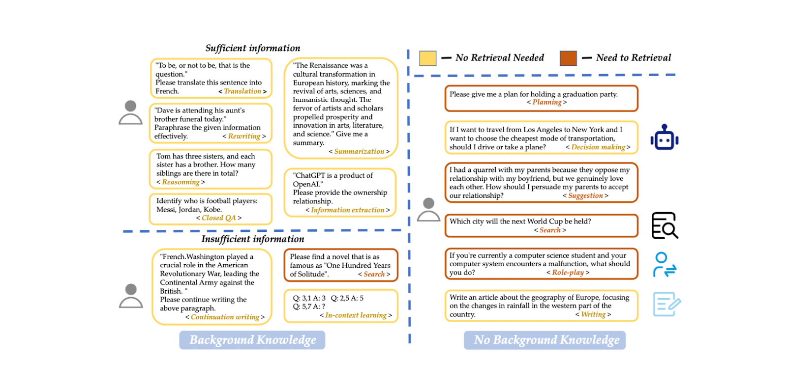Figure- Query classification dataset example..png

Figure: Query classification dataset example. Source

In the paper, a BERT-base-multilingual model is used for query classification. The training data includes 15 types of prompts in total, such as translation, summarization, rewriting, in-context learning, etc. There are two distinct labels: "sufficient" if the prompt is entirely based on user-given information and doesn't need retrieval, and "insufficient" if the prompt information is incomplete, needs specialized information, and requires a retrieval process. Using this approach, the model achieved 95% in both accuracy and F1 score.

This query classification step can significantly improve the efficiency of the RAG process by avoiding unnecessary retrievals for queries that can be handled directly by the LLM. It acts as a filter, ensuring that only queries requiring additional context are sent through the more time-consuming retrieval process.

Figure- Query classifier result..png

Figure: Query classifier result. Source

Chunking Technique

Chunking refers to the process of splitting long input documents into smaller segments. This process is highly useful in providing the LLM with a more granular context. There are several methods for chunking, including token-level and sentence-level approaches. Sentence-level chunking often leads to a good balance between simplicity and semantic preservation of the context. When choosing a chunking method, we need to be careful with the chunk size, as chunks that are too short may not provide helpful context for the LLM.

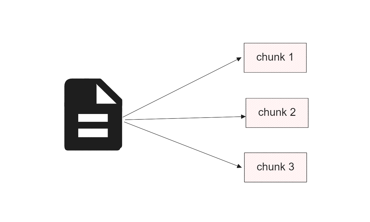Figure- Splitting a long document into smaller chunks.png

Figure: Splitting a long document into smaller chunks

To find the optimal chunk size, an evaluation was conducted on the Lyft 2021 document. The first 60 pages of the document were chosen as a corpus and chunked into several sizes. An LLM was then used to generate 170 queries based on these 60 pages. The text-embedding-ada-002 model was used for embeddings, while the Zephyr 7B model was used as the LLM to generate responses based on the chosen queries.

To evaluate the model's performance on different chunk sizes, GPT-3.5 Turbo was used. Two metrics were employed to evaluate the response quality: faithfulness and relevancy. Faithfulness measures whether the response is hallucinated or matches the retrieved contexts, while relevancy measures whether the retrieved contexts and responses match the queries.

Figure- Comparison of different chunk sizes. .png

Figure: Comparison of different chunk sizes. Source

The results show that a maximum chunk size of 512 tokens is preferred for highly relevant response generation from the LLM. Shorter chunk sizes, such as 256 tokens, also perform well and can improve the overall runtime of the RAG application. Advanced chunking techniques such as small2big and sliding windows can be used to combine the benefits of different chunk sizes.

Small2big is a chunking approach that organizes chunk block relationships. Small-sized chunks are used to match queries, and larger chunks containing the information from the smaller ones are used as the final context for the LLM. A sliding window is a chunking method that provides token overlaps between chunks to preserve context information.

Figure- Comparison of different chunking techniques..png

Figure: Comparison of different chunking techniques. Source

Experiments show that with a smaller chunk size of 175 tokens, a larger chunk size of 512 tokens, and a chunk overlap of 20 tokens, both chunking techniques improve the faithfulness and relevancy scores of the LLM responses.

Next, finding the best embedding model to represent each chunk as a vector embedding is crucial. A test on namespace-Pt/msmarco was conducted for this purpose. The results show that both LLM Embedder and bge-large-en models perform best. However, since LLM Embedder is three times smaller than bge-large-en, it was chosen as the default embedding for the experiment.

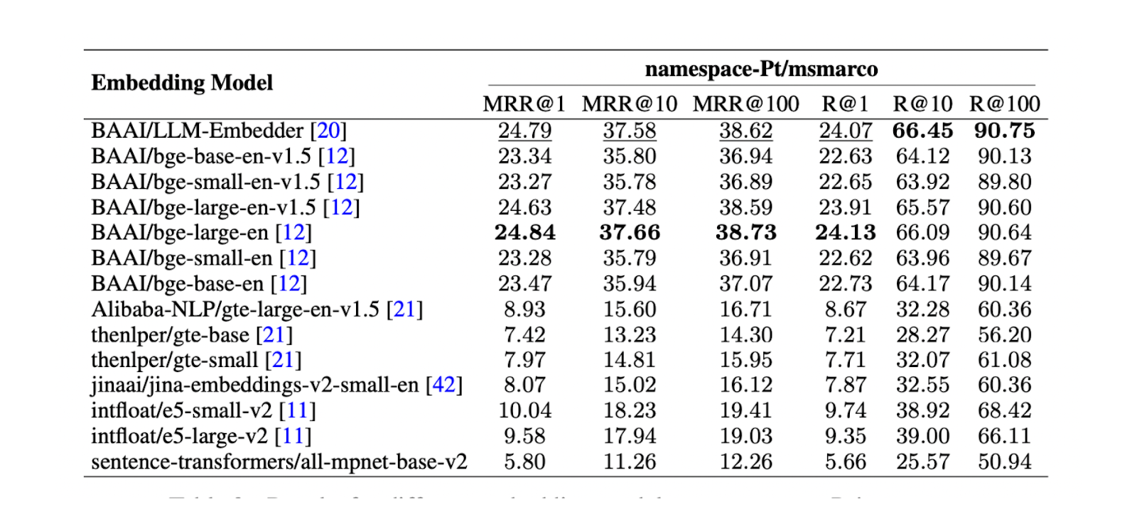Figure- Results for different embedding models on namespace-Pt:msmarco. .png

Figure: Results for different embedding models on namespace-Ptmsmarco. Source

Vector Databases

Vector databases play a crucial role in RAG applications, particularly in storing and retrieving relevant contexts. In common real-world RAG applications, we deal with a huge amount of documents, leading to a vast number of context embeddings that need to be stored. In such cases, storing these embeddings in local memory is insufficient, and computing the retrieval of relevant contexts among large collections of embeddings would take considerable time.

Vector databases are designed to solve these problems. With a vector database, we can store millions to even billions of vector embeddings and perform context retrieval in a split second. When choosing the best vector database for your use case, we need to consider several factors, such as index type support, billion-scale vector support, hybrid search support, and cloud-native capabilities.

Among these criteria, Milvus stands out as the best open-source vector database compared to its competitors like Weaviate, Chroma, Faiss, Qdrant, etc.

Comparison of Various Vector Databases..png

Comparison of Various Vector Databases. Source.

In terms of index type support, Milvus offers several indexing methods to suit various needs, such as the naive flat index (FLAT) or other indexing types designed to speed up the retrieval process, like the inverted file index (IVF-FLAT) and Hierarchical Navigable Small World (HNSW). To compress the memory needed to store the contexts, you can also implement product quantization (PQ) during the embeddings' indexing process.

Milvus also supports a hybrid search approach. This approach enables us to combine two different methods during the context retrieval process. For example, we can combine dense embedding with sparse embedding to retrieve relevant contexts, enhancing the relevancy of the retrieved context with respect to the query. This, in turn, also enhances the response generated by the LLM. Additionally, we can combine dense embedding with metadata filtering if desired.

If you want to use Milvus on the cloud, whether on GCP or AWS, to store billions of embeddings, you can opt for its managed service: Zilliz Cloud.

With Zilliz Cloud, you can create cluster units (CUs) optimized for both capacity and performance to store large-scale embeddings. For example, you can create 256 performance-optimized CUs serving 1.3 billion 128-dimensional vectors or 128 capacity-optimized CUs serving 3 billion 128-dimensional vectors.

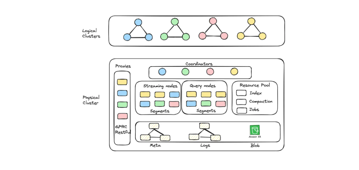Diagram of logical cluster and auto-scaling implemented in Zilliz Cloud Serverless..png

Diagram of logical cluster and auto-scaling implemented in Zilliz Cloud Serverless.

If you'd like to build a RAG application with Milvus but also want to save on operating costs, you can opt for Zilliz Cloud Serverless. This service provides an auto-scaling feature within Milvus, with costs that increase only as your business grows. The serverless option is also perfect for cost savings because you only pay when you use the service, not when it's idle.

Zilliz Cloud has launched multiple exciting updates recently, including a new migration service, multiple replicas, new integration with Fivetran connectors, auto-scaling capability, and many more production readiness features. See more details below:

Retrieval Techniques

The main goal of the retrieval component is to fetch the top k most relevant contexts for a given query. However, a significant challenge in this component that might affect the overall quality of our RAG comes from the query itself. Original queries are often poorly written or expressed, lacking the semantic information needed for RAG applications to fetch relevant contexts.

Several commonly applied techniques to solve this problem include:

Query rewriting: Prompts the LLM to rewrite the original query to improve its clarity and semantic information.
Query decomposition: Decomposes the original query into subqueries and performs retrieval based on these sub-queries.
Pseudo-document generation: Generates hypothetical or synthetic documents based on the original query and then uses these hypothetical documents to retrieve similar documents in the database. The most well-known implementation of this approach is HyDE (Hypothetical Document Embeddings).

Experiments show that combining HyDE and hybrid search yields the best results on TREC DL19/20 compared to query rewriting and query decomposition. The hybrid search mentioned in the experiment combines LLM Embedder to obtain dense embeddings and BM25 to obtain sparse embeddings.

The workflow of HyDe + hybrid search is as follows: first, we generate a hypothetical document that answers the query with HyDE. Next, this hypothetical document is concatenated with the original query before being transformed into dense and sparse embeddings using LLM Embedder and BM25, respectively.

Results for different retrieval methods. .png

Results for different retrieval methods. Source

Although the combination of HyDE and hybrid search yields the best results, it also comes with higher computational costs. Based on further tests on several NLP datasets, both hybrid search and using only dense embeddings result in comparable performance to HyDE + hybrid search, but with almost 10x lower latency. Therefore using a hybrid search would be more recommended.

Since we're using a hybrid search, the retrieved contexts are based on vector search from dense and sparse embeddings. Therefore, it's also interesting to examine the impact of the weighting value between dense and sparse embeddings on the overall relevance score according to this equation:

formula.png

Figure- Results of hybrid search with different alpha values..png

Figure: Results of hybrid search with different alpha values. Source.

The experiment shows that a weighting value of 0.3 yields the best overall relevance score on TREC DL19/20.

Reranking and Repacking Techniques

The main goal of reranking techniques is to reorder the top k most relevant contexts fetched from the retrieval method to ensure that the most similar context is returned at the top of the list. There are two common approaches to rerank the contexts:

DLM Reranking: This method uses a deep learning model for reranking. The model is trained with a pair consisting of the original query and a context as input and a binary label "true" (if the pair is relevant to each other) or "false" as output. The contexts are then sorted based on the probability the model returns when it predicts a pair of queries and context as "true."
TILDE Reranking: This approach uses the likelihood of each term in the original query to rerank. During inference time, we can use either the query likelihood component (TILDE-QL) alone for faster reranking or the combination of TILDE-QL with its document likelihood component (TILDE-DL) to improve the reranking result at a higher computational cost.

Figure- Results of different reranking methods..png

Figure: Results of different reranking methods. Source

Experiments on the MS MARCO Passage ranking dataset show that the DLM reranking method with the Llama 27B model yields the best reranking performance. However, since it's a large model, using it comes with a significant computational cost. Therefore, using mono T5 is more recommended for DLM reranking, as it provides a balance between performance and computational efficiency.

After the reranking phase, we also need to consider how to present the reranked contexts to our LLM: whether in descending ("forward") or ascending ("reverse") order. Based on the experiments conducted in this paper, it can be concluded that the best response quality is generated using the "reverse" configuration. The hypothesis is that positioning more relevant context closer to the query leads to optimal outcomes.

Summarization Techniques

In cases where we have long contexts retrieved from previous components, we might want to make them more compact and remove redundant information. To achieve this goal, summarization approaches are typically implemented.

There are two different context summarization techniques: extractive and abstractive.

Extractive summarization splits the input document into smaller segments, then ranked based on importance. Meanwhile, the abstractive method generates a new context summary that contains only relevant information.

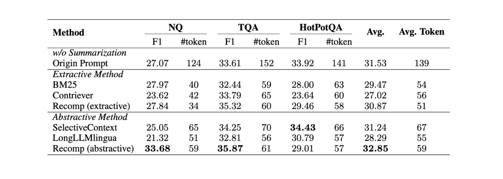Figure- Comparison between different summarization methods..png

Figure: Comparison between different summarization methods. Source

Based on experiments on three different datasets (NQ, TriviaQA, and HotpotQA), abstractive summarization with Recomp yields the best performance compared to other abstractive and extractive methods.

The Summary of Best RAG Techniques

Now that we know the best approach for each RAG component for specific benchmark datasets, we can further test all of the approaches mentioned in the previous sections on more datasets. The results show that each component contributes to the overall performance of our RAG application. Below is a summary of the results for each approach in each component based on five different datasets:

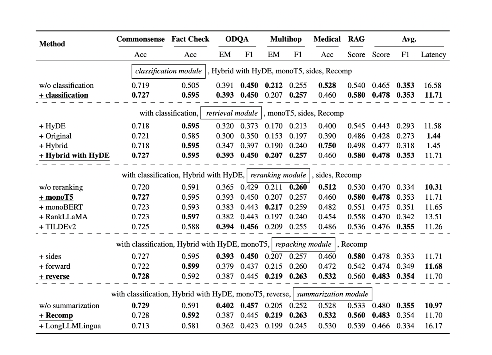Figure- Results of the search for optimal RAG practices..png

Figure: Results of the search for optimal RAG practices. Source

The query classification component proves to help improve the accuracy of responses and reduce the overall runtime latency. This initial step helps determine whether a query requires context retrieval or can be processed directly by the LLM, thus optimizing the system's efficiency.

The retrieval component is crucial in ensuring that we obtain relevant context candidates with respect to the query. For this component, a more scalable and performant vector database like Milvus or its managed service, Zilliz Cloud, is recommended. In addition, hybrid search or dense embedding search is recommended. These methods strike a balance between comprehensive context matching and computational efficiency.

The reranking component ensures we get the most relevant contexts by reordering the top k contexts retrieved from the retrieval component. The monoT5 model is recommended for reranking due to its balance of performance and computational cost. This step refines the selection of contexts, prioritizing the most relevant contexts to the query.

The reverse method is recommended to repack the context. This approach positions the most relevant context closest to the query, potentially leading to more accurate and coherent responses from the LLM.

Finally, the abstractive method with Recomp has shown the best performance for context summarization. This technique helps condense long contexts while preserving key information, making it easier for the LLM to process and generate relevant responses.

LLM Fine-Tuning

In most cases, LLM fine-tuning is not necessary, especially if you're using a performant LLM with many parameters. However, if you have hardware constraints and can only use smaller LLMs, you may need to fine-tune them to make them more robust when generating responses related to your use case. Before fine-tuning an LLM, you need to consider the data you will use as training data.

During the data preparation, you can collect training data in prompt and context as a pair of inputs, with an example of generated text as output. Experiments show that augmenting your data with a mix of relevant and randomly selected contexts during training will result in the best performance. The intuition behind this is that mixing relevant and random contexts during fine-tuning can improve our LLM's robustness.

Conclusion

In this article, we explored various RAG components, from query classification to context summarization. We have discussed and highlighted the approaches with optimal performance in each component.

These optimized components work together to improve the overall performance of the RAG system. They’re improving the quality and relevance of generated responses while maintaining computational efficiency. By implementing these best practices in each component, we can create a more robust and effective RAG system capable of handling a wide range of queries and tasks.