Understanding HNSWlib: A Graph-based Library for Fast Approximate Nearest Neighbor Search
HNSWlib is an open-source C++ and Python library implementation of the HNSW algorithm, which is used for fast approximate nearest neighbor search.
Read the entire series
- Raft or not? The Best Solution to Data Consistency in Cloud-native Databases
- Understanding Faiss (Facebook AI Similarity Search)
- Information Retrieval Metrics
- Advanced Querying Techniques in Vector Databases
- Popular Machine-learning Algorithms Behind Vector Searches
- Hybrid Search: Combining Text and Image for Enhanced Search Capabilities
- Ensuring High Availability of Vector Databases
- Ranking Models: What Are They and When to Use Them?
- Navigating the Nuances of Lexical and Semantic Search with Zilliz
- Enhancing Efficiency in Vector Searches with Binary Quantization and Milvus
- Model Providers: Open Source vs. Closed-Source
- Embedding and Querying Multilingual Languages with Milvus
- An Ultimate Guide to Vectorizing and Querying Structured Data
- Understanding HNSWlib: A Graph-based Library for Fast Approximate Nearest Neighbor Search
- What is ScaNN (Scalable Nearest Neighbors)?
- Getting Started with ScaNN
- Next-Gen Retrieval: How Cross-Encoders and Sparse Matrix Factorization Redefine k-NN Search
- What is Voyager?
- What is Annoy?
Vector search, also known as vector similarity search, is one of the most important techniques in the modern era of AI. Whether we want to build a recommendation system or advanced Gen AI applications like Retrieval Augmented Generation (RAG), we'll definitely need to perform vector search during the process.
Among other factors, the most important aspects of vector search are accuracy and speed. Accuracy is needed to ensure we get the most relevant results based on our query, while speed is necessary to obtain these results quickly. The k-Nearest Neighbors (kNN) algorithm is the most commonly implemented method for vector searches. As the name suggests, with kNN, the data point nearest to the query will be chosen as the most relevant result. However, the main problem with this algorithm is its speed, especially when dealing with millions of data points.
In this article, we're going to discuss a vector search library called HNSWlib. This library implements an algorithm called HNSW to perform vector search more efficiently. Before we talk about HNSWlib in more detail, let's first learn what vector search is.
Introduction to Vector Search
Vector search is a method commonly used in information retrieval to find the most similar information from large collections of unstructured data (images, documents, audio, etc) to a given query. As the name suggests, both the documents and the query are represented as vectors with a specific dimension in a high-dimensional vector space. The dimension of the vector depends on the embedding model used to transform the documents and query. For example, if we use "all-MiniLM-L6-v2" as an embedding model, we get a vector of 384 dimensions for each query or document.
As you might already know, the vectors produced by embedding models contain the semantic meaning of the documents they represent. Therefore, the vectors of similar documents are placed close to each other in the vector space, as you can see in the 2D visualization below:
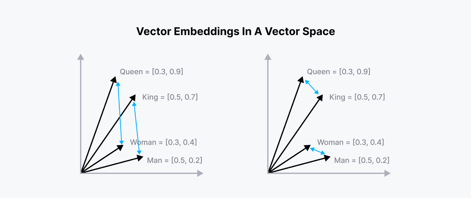 Vector embeddings of similar words in a 2D vector space..png
Figure: Vector embeddings of similar words in a 2D vector space.
To find the most similar documents to a given query, we can compute the similarity or the distance between a query vector and all vectors in the document collection. The document vector with the highest similarity score (or lowest distance) to the query vector is then picked as the most similar document. This is the intuition behind vector search.
The k-Nearest Neighbors (kNN) search is a fundamental operation in vector search, but it can become computationally expensive with large datasets when performed as a brute-force linear scan. To optimize kNN search performance, various indexing algorithms have been developed, with Hierarchical Navigable Small World (HNSW) being one of the most effective. Let's examine how basic kNN search works before exploring how HNSW makes it more efficient, especially for large-scale applications.
Brief Introduction to k-Nearest Neighbors (kNN)
During the vector search operation, the kNN algorithm calculates the similarity of our query vector with each document vector in the database. If we have 100 documents in memory, the kNN algorithm will calculate the similarity or distance of our query vector with each of the 100 document vectors. In other words, the kNN algorithm performs an exhaustive search and therefore guarantees an exact vector search result, i.e., we'll get the most similar document as the output.
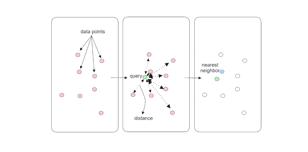 The kNN algorithm workflow..png
Figure: The kNN algorithm workflow.
However, the exhaustive search performed by the kNN algorithm comes with an obvious drawback: speed. The time complexity of the vector search operation using this algorithm grows linearly with the number of documents stored in our memory. The more documents we have in the memory, the longer it takes to complete a vector search operation. This drawback becomes more and more apparent as we accumulate millions of documents.
HNSW (Hierarchical Navigable Small Worlds) is one of the advanced vector search methods designed to solve this problem. We’ll see in the next section how this algorithm can balance between the speed and accuracy result of a vector search operation.
Skip List and NSW as HNSW Foundation
HNSW is a graph-based vector search algorithm that enables fast vector search operations. It relies on two key concepts: skip lists and Navigable Small World (NSW) graphs. Therefore, we need to understand the fundamentals of these two concepts before we can understand how the HNSW algorithm works.
A skip list is a probabilistic data structure that consists of multiple layers of linked lists, where the higher the layer, the more elements in the list are skipped. As you can see in the visualization below, the lowest layer contains all of the elements in a linked list. As we move towards the higher layers, the linked lists progressively skip more and more elements, resulting in lists with fewer elements.
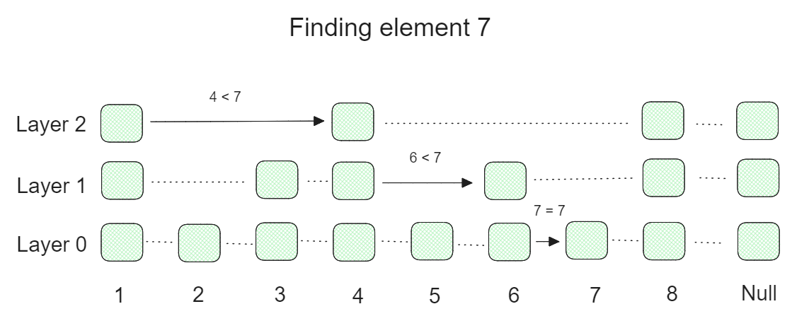 Skip list workflow to find a particular element..png
Figure: Skip list workflow to find a particular element.
The above visualization shows an example of how the searching process for a particular element is performed.
Let's say we're trying to find element 7 from a skip list with 3 layers and 8 elements in the original linked list. First, we start from the highest layer and check if the first element is below 7. If yes, then we check the second element. If the second element is above 7, then we use the first element as a starting point in the lower layer. Next, we do the exact same thing in the lower layer and gradually descend to the lowest layer to find the desired element. The skipping process over many elements makes skip lists really fast when performing a search operation.
Now that we understand the fundamental concept of a skip list, let's talk about NSW graphs. In a nutshell, an NSW graph is built by randomly shuffling a collection of data points and then inserting them one by one. After each insertion, each data point is connected to its nearest neighbors through a predefined number of edges (M). When each point is connected to its nearest neighbors, it creates a "small world" phenomenon, where any two points can be traversed with relatively short paths.
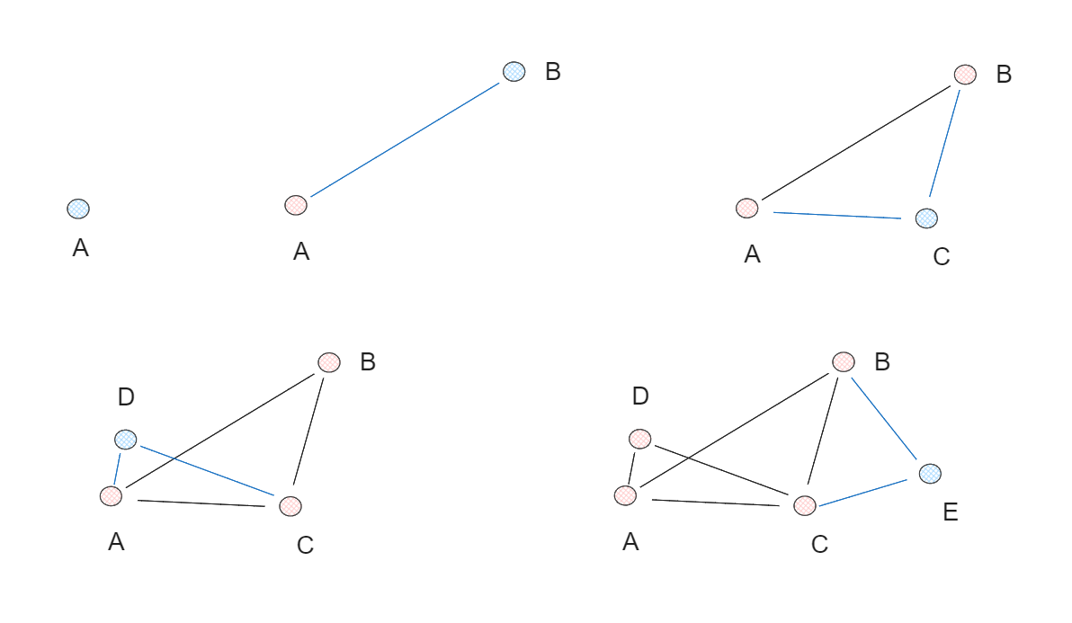 NSW graph creation process..png
Figure: NSW graph creation process.
In the above example, we create an NSW graph from 5 data points and set the number of edges (M) to be 2. In each iteration, one data point is inserted into the graph individually, and two of each point's nearest neighbors are connected via an edge.
The Concept of HNSW
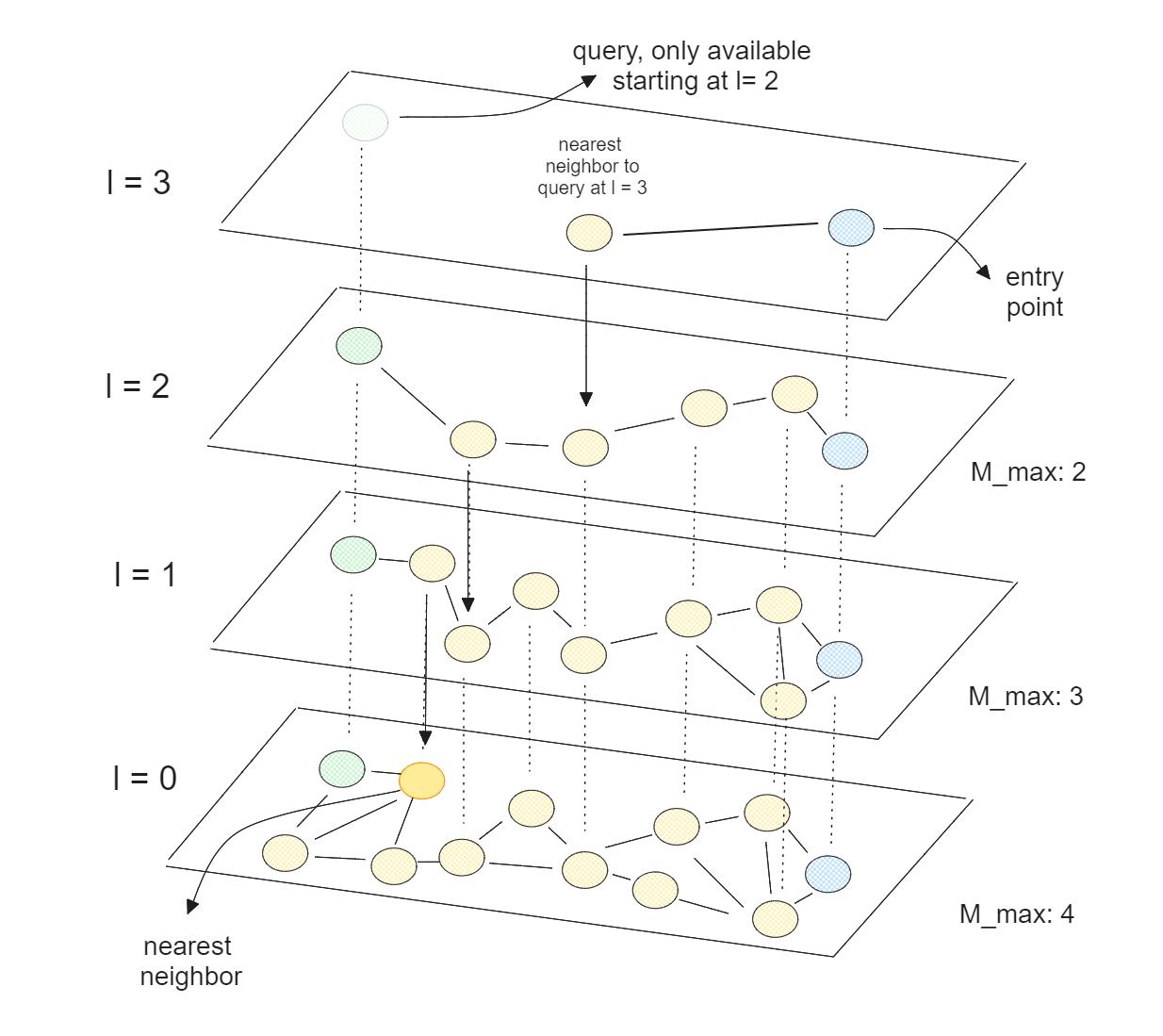
HNSW combines the concepts of skip lists and NSW graphs discussed above. Instead of just one graph, HNSW consists of several layers of graphs, forming a hierarchy. Similar to the skip list concept, the lowest layer of the graph contains all of the elements, and the higher the layer, the more elements are skipped.
During the graph creation process, HNSW starts by assigning a random number from 0 to l to each element, where l is the maximum layer in which an element can be present in a multi-layered graph. If an element has l equal to 2 and the total number of layers is 4, this element will be present from layer 0 up to layer 2 but not in layer 3.
 Vector search using HNSW algorithm..png
Figure: Vector search using HNSW algorithm.
During the vector search process, the HNSW algorithm first selects an entry point, which should be the element present at the highest layer. Next, the nearest neighbor of the entry point is picked, and it checks if this nearest neighbor brings us closer to the query point. If yes, and no other elements in the highest layer are closer to the query point, then the same searching procedure continues in the lower layer. Note that it will use the chosen nearest neighbor of our entry point as the new entry point in the lower layer, as you can see in the visualization above.
Key Features of HNSW
The HNSW algorithm relies on a multi-layered graph concept, where the higher the layer, the fewer elements are present. This, in turn, speeds up the searching process during vector search operations, as we don't need to traverse through unpromising elements before finding the nearest point to our query point.
High recall is possible, however, an exact match is not guaranteed because HNSW skips some elements during the search process. This applies not only to HNSW but also to other Approximate Nearest Neighbors (ANN) approaches such as FAISS or ScaNN. Therefore, HNSW is not an ideal algorithm to implement if your use case demands an exact matching result.
If an exact matching result is not a requirement but you still want to obtain an accurate result, we can easily tune the hyperparameters of HNSW during both graph creation time and search time:
M: The number of edges per element during the graph creation in each layer. A higherMvalue generally results in better search accuracy, but it comes at the cost of slower index-building time.efConstruction: The number of neighbors considered to find the nearest neighbor at each layer during graph creation. The more neighbors considered, the better the index quality, but the slower the index building time will be.efSearch: The number of nearest neighbors to consider during the vector search process. The higher theefSearch, the higher the recall, but the searching process will be slower.
Aside from the speed vs. accuracy trade-off, we also need to pay attention to memory consumption during the graph creation process. This is because HNSW requires the entire dataset to be loaded into RAM, which can be a problem if your dataset is too large to fit into memory.
As you can imagine, the higher the M value, the more memory we need to allocate to store the information of each element's neighbors. Also, the memory grows linearly as the combination of elements and their dimensions are added to the graph. Therefore, fine-tuning both M and efConstruction is crucial during the graph creation process, especially in large-scale applications.
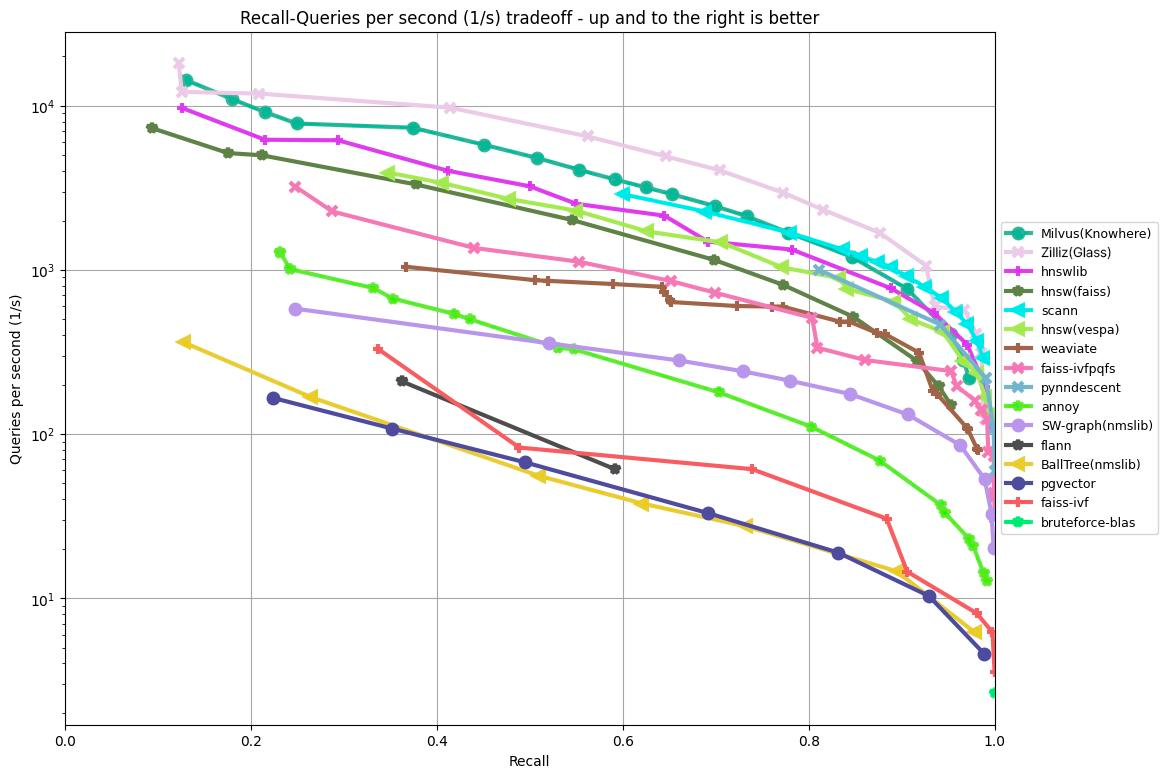
Regardless of the memory consumption, the performance of HNSW on large datasets is very competitive compared to other ANN methods. As you can see in the ANN benchmark on the GIST1M dataset (1M vectors with 960 dimensions) below, HNSW, following Milvus’ Knowhere and Zilliz Cloud’s Glass algorithms, achieved a top-three result among a wide selection of other methods, such as FAISS, Annoy, pgvector, etc.
 ANN Benchmark results on the GIST1M dataset.png
Figure: ANN Benchmark results on the GIST1M dataset
HNSWlib Implementation and Its Integration with Milvus
HNSWlib is an open-source C++ and Python library implementation of the HNSW algorithm. It provides a practical and optimized way to use the HNSW algorithm in real-world applications. The library is designed to be highly efficient, making it suitable for use cases involving large-scale data.
HNSWlib is perfect for building a simple prototype for your vector search use case. However, when you want to perform vector search in more complicated scenarios with 100 million, or even billions of data points, HNSWlib wouldn't be an optimal solution.
Like other vector search libraries, HNSWlib is a lightweight ANN library with limited functionality. For example, as your data points grow larger and larger, using HNSWlib wouldn't scale well. If you have millions of data points, using HNSWlib wouldn't be feasible as the memory consumption would be too high to fit into RAM. In a large-scale application, utilizing a vector database like Milvus would be the way to go.
A vector database is a full-fledged solution that enables you to efficiently store massive amounts of data and perform effective vector searches on them. Milvus, for example, supports cloud-native and multi-tenancy services, which allow you to store, index, and retrieve millions or even billions of data points from several users on the cloud. Vector search libraries like HNSWlib are usually integrated into vector databases to perform fast vector searches on the stored data.
In this section, we'll show you how to implement HNSWlib as a standalone vector search library and how to use it when integrated into the Milvus vector database. Let's start with an example of the native implementation of HNSWlib.
To install HNSWlib, you can do it via pip install:
pip install hnswlib
Next, let’s create 100 dummy data points, each has a dimension of 128. Next, we build the HNSW graph with M of 8 and efConstruction of 25. Finally, we calculate the nearest neighbor of a query data point.
import hnswlib
import numpy as np
import pickle

dim = 128
num_elements = 100

# Generating sample data
data = np.float32(np.random.random((num_elements, dim)))
ids = np.arange(num_elements)

# Generating query point
query = np.float32(np.random.random((1, dim)))

# Declaring index
p = hnswlib.Index(space = 'l2', dim = dim) # possible options are l2, cosine or ip

# Initializing index - the maximum number of elements should be known beforehand
p.init_index(max_elements = num_elements, ef_construction = 25, M = 8)

# Element insertion (can be called several times):
p.add_items(data, ids)

# Controlling the recall by setting ef:
p.set_ef(50) # ef should always be > k

# Query dataset, k - number of the closest elements (returns 2 numpy arrays)
labels, distances = p.knn_query(query, k = 1)
And that’s all we have to do to implement the native HNSWlib.
Next, let’s see how we can utilize HNSW integration in Milvus. The easiest way to get started with Milvus is through Milvus Lite (a lightweight version of Milvus and can be imported into your Python app), and we can install it with pip install.
!pip install -U pymilvus
!pip install pymilvus[model]
Now we can start by creating a collection and defining its indexing method. First, we define a collection schema, then specify HNSW as the indexing method, and Milvus will automatically use HNSW under the hood. Then, we can start inserting data into the collection for index building.
from pymilvus import MilvusClient, DataType
from pymilvus import model

client = MilvusClient("demo.db")

# 1. Create schema
schema = MilvusClient.create_schema(
    auto_id=False,
    enable_dynamic_field=False,
)

# 2. Add fields to schema
schema.add_field(field_name="id", datatype=DataType.INT64, is_primary=True)
schema.add_field(field_name="vector", datatype=DataType.FLOAT_VECTOR, dim=768)
schema.add_field(field_name="text", datatype=DataType.VARCHAR, max_length=200)

# 3. Prepare index parameters
index_params = client.prepare_index_params()

# 4. Add indexes
index_params.add_index(
    field_name="vector",
    index_type="HNSW",
    metric_type="L2"
)

# Create collection
if client.has_collection(collection_name="demo_collection"):
    client.drop_collection(collection_name="demo_collection")

client.create_collection(
    collection_name="demo_collection",
    schema=schema,
    index_params=index_params
)

# Define embedding model
embedding_fn = model.DefaultEmbeddingFunction()

# Text data to search from.
docs = [
    "Artificial intelligence was founded as an academic discipline in 1956.",
    "Alan Turing was the first person to conduct substantial research in AI.",
    "Born in Maida Vale, London, Turing was raised in southern England.",
]

# Transform text data into embeddings
vectors = embedding_fn.encode_documents(docs)

data = [
    {"id": i, "vector": vectors[i], "text": docs[i]}
    for i in range(len(vectors))
]

# Insert embeddings into Milvus
res = client.insert(collection_name="demo_collection", data=data)

Finally, if we want to perform vector search, we can do the following:

SAMPLE_QUESTION = "What's Alan Turing achievement?"
query_vectors = embedding_fn.encode_queries([SAMPLE_QUESTION])

res = client.search(
    collection_name="demo_collection",
    data=query_vectors,
    limit=1,
    output_fields=["text"],

)

context = res[0][0]["entity"]["text"]
Conclusion
Vector search implementation is very important in modern AI applications. The demand for both accuracy and speed in these applications necessitates the development of sophisticated vector search algorithms. While the kNN algorithm provides highly accurate results through exhaustive searching, its linear time complexity makes it impractical for large-scale datasets.
The HNSW algorithm offers an innovative solution to this limitation by balancing speed and accuracy, using multi-layered graph structures. By combining skip lists and NSW graphs, HNSW enables fast, approximate searches that can handle massive datasets efficiently. The flexibility to fine-tune hyperparameters like M, efConstruction, and efSearch further allows HNSW to be adapted to a variety of use cases, depending on the specific trade-offs between search speed, accuracy, and memory consumption required by each application.
HNSWlib is an open-source C++ and Python library that simplifies the implementation of the HNSW algorithm. It provides a practical and optimized way to use the algorithm in real-world applications. The library is designed to be highly efficient, making it suitable for use cases involving large-scale data.
Check out this handle table comparing HNSW to some of the other popular vector indexes.
 comparing different index.png
Frequently Asked Questions
What is HNSWlib?
HNSWlib is a library for vector search. It implements the HNSW algorithm, which creates a hierarchical graph structure for efficient similarity search in high-dimensional spaces. Due to its excellent balance of speed and accuracy, it's widely adopted in vector databases and particularly popular in applications like vector search, recommendation systems, and image retrieval.
How does HNSWlib compare to other ANN libraries like Faiss?
HNSWlib generally offers better search performance than many other ANN libraries for most use cases, especially when high recall is required. Also, HNSWlib focuses on implementing a single algorithm (HNSW) exceptionally well. HNSWlib is often simpler to use but may consume more memory than some Faiss indexes.
What are the memory requirements for HNSWlib?
HNSWlib's memory usage is typically higher than other ANN libraries because it needs to store the graph structure in memory. The memory consumption depends on the number of elements (N), dimension (D), and the M parameter (maximum number of connections per element).
What are the pros and cons of HNSWlib?
It provides exceptional search speed with logarithmic complexity O(log N) and high recall rates, and it supports dynamic updates for adding new data without rebuilding the index. However, the main cons include higher memory consumption compared to other ANN algorithms since it needs to store the entire graph structure in memory, slower index construction time, especially for large datasets, and lack of native support for element deletion.
What parameters should I tune in HNSWlib for optimal performance?
The two most important parameters in HNSWlib are M (number of edges per data point) and ef_construction (number of nearest neighbors considered during construction). Higher values for both parameters generally lead to better recall but increased memory usage and construction time. The good thing is that another hyperparameter (ef_search) can be tuned at query time to balance search speed and accuracy.
Further Resources
- Introduction to Vector Search
- Brief Introduction to k-Nearest Neighbors (kNN)
- Skip List and NSW as HNSW Foundation
- The Concept of HNSW
- Key Features of HNSW
- HNSWlib Implementation and Its Integration with Milvus
- Conclusion
- Frequently Asked Questions
- Further Resources
Content
Start Free, Scale Easily
Try the fully-managed vector database built for your GenAI applications.
Try Zilliz Cloud for FreeKeep Reading

Raft or not? The Best Solution to Data Consistency in Cloud-native Databases
Explain why consensus-based algorithms like Paxos and Raft are not the silver bullet and propose a solution to consensus-based replication.

Understanding Faiss (Facebook AI Similarity Search)
Faiss (Facebook AI similarity search) is an open-source library for efficient similarity search of unstructured data and clustering of dense vectors.

Ranking Models: What Are They and When to Use Them?
Explore different ranking algorithms, their usage, and best practices. Uncover the real-world success stories of ranking algorithms and their evolution over time.


