


What is the K-Nearest Neighbors (KNN) Algorithm in Machine Learning?
Latest Update: March 1, 2025
By the end of this article, you will be able to:
Explain the fundamental principles behind KNN and how it works
Select appropriate distance metrics for different types of data
Implement KNN for both classification and regression tasks
Optimize KNN models by selecting the ideal value of k
Understand the limitations of KNN and when to use alternative approaches
Apply KNN to real-world problems with Python
Introduction: Similarity in Everyday Decision Making
Imagine you’re trying to decide which restaurant to visit in a new city. What do you typically do? You might ask friends with similar tastes to yours for recommendations, trusting that if people with preferences similar to yours enjoyed a restaurant, you likely will too.
This intuitive concept—that items or entities similar to each other often share important characteristics—is precisely what powers the K-Nearest Neighbors (KNN) algorithm. KNN formalizes this intuition into a powerful machine learning technique that has applications across numerous domains, from recommendation systems to medical diagnosis.
The knn algorithm is a supervised machine learning algorithm that can solve both classification and regression problems. It estimates the likelihood that a data point will belong to one group or another based on which existing data points are closest to it. Unlike many ml algorithms that build complex models, KNN’s elegance lies in its simplicity: the algorithm simply stores the training data and makes predictions by finding the most similar examples.
Definition of KNN
The K-nearest neighbor algorithm is a supervised machine learning algorithm that leverages proximity to make classifications or predictions about the grouping of an individual data point. As a non-parametric, lazy learning algorithm, KNN stores the entire training dataset and performs computations only at the time of classification. This means that instead of building a model during a training phase, KNN makes predictions by directly comparing new data points to the stored training data. The algorithm is versatile, being used for both classification and regression tasks, and its performance is influenced by the choice of K (the number of nearest neighbors considered) and the distance metric used to measure similarity.
Importance of KNN in Data Science
The KNN algorithm holds a significant place in the realm of ml and data science due to its simplicity, ease of interpretation, and relatively low computational cost for small to medium-sized datasets. Its straightforward approach makes it an excellent starting point for beginners in data science, while its effectiveness ensures it remains a valuable tool for seasoned professionals. KNN is widely applied across various domains, including image classification, text classification, and recommendation systems. For instance, it can predict user churn in a streaming service, assist in medical diagnosis, and aid in financial forecasting. Its ability to handle non-linear relationships and robustness to outliers further enhance its appeal, making it a popular choice in the industry.
Foundational Concepts
Supervised vs. Unsupervised Learning
KNN belongs to the family of supervised learning algorithms, meaning it requires labeled training data to make predictions. In supervised learning, the algorithm learns from examples where the correct answers (labels) are provided, in contrast to unsupervised learning where the algorithm must find patterns in unlabeled data.
Lazy vs. Eager Learning
What makes KNN unique among many ml algorithms is that it's considered a "lazy learner." Most algorithms go through an explicit training phase to build a model before making predictions. KNN, however, doesn't have a distinct training phase—it simply stores the training dataset and delays all computation until prediction time. This is why KNN is also called:
Instance-based learning
Memory-based learning
Non-parametric learning
Since KNN doesn't make assumptions about the underlying data distribution (non-parametric) and doesn't summarize the training data into a compact model, it can capture complex decision boundaries that parametric models might miss.
Classification vs. Regression with KNN
KNN can be used for both classification and regression tasks:
KNN Classification: Predicts the class label of a new instance by finding the most common class among its k nearest neighbors. The classification of a new data point is based on the most common class among its k nearest neighbors (KNN).
KNN Regression: Predicts the numerical value of a new instance by averaging the values of its k nearest neighbors.
Feature Space and Similarity
The cornerstone of KNN is the concept of similarity or distance in feature space. Each data point is represented as a vector in a multi-dimensional space, where each dimension corresponds to a feature. The similarity between two data points is inversely related to the distance between them in this feature space—the closer two points are, the more similar they are considered to be.
Distance Metrics in Depth
The choice of distance metric is crucial in KNN as it directly affects which points are considered "nearest" to each other. Different distance metrics are appropriate for different types of data and problem domains.

Euclidean Distance
The Euclidean distance is the true straight-line distance between two points in Euclidean space. It's the most commonly used distance metric in KNN.
Mathematical formula:
Where x and y are two points in n-dimensional space.
When to use: Euclidean distance works well when the data is continuous and has meaningful relationships in all dimensions. It's especially appropriate when features are measured on similar scales.
Manhattan Distance
Also known as city block or L1 distance, Manhattan distance calculates the sum of the absolute differences between the coordinates of two points. In the KNN algorithm, Manhattan distances are used to measure the proximity of data points in grid-like structures, making it particularly suitable for such environments.
Mathematical formula:
When to use: Manhattan distance is useful when features represent discrete or binary attributes, or when the feature space is grid-like. It can be less sensitive to outliers than Euclidean distance.
Cosine Similarity
Cosine similarity measures the cosine of the angle between two vectors, focusing on orientation rather than magnitude.
Mathematical formula:
When to use: Cosine similarity is particularly useful for text analysis and high-dimensional sparse data, where the magnitude of vectors may not be as important as their direction.
Hamming Distance
Hamming distance counts the number of positions at which corresponding elements differ in two sequences of equal length.
Mathematical formula: For two strings of equal length, the Hamming distance is the number of positions at which the corresponding symbols differ.
When to use: Hamming distance is ideal for categorical data or when working with binary features. It's commonly used in information theory, coding theory, and for comparing strings or bit vectors.
Guidelines for Choosing Distance Metrics
Euclidean distance: Continuous data with similar scales
Manhattan distance: Grid-like spaces, feature independence
Cosine similarity: Text data, sparse high-dimensional data
Hamming distance: Categorical data, binary features
Remember that regardless of which distance metric you choose, feature scaling is often necessary to prevent features with larger scales from dominating the distance calculations.
The KNN Algorithm: Step by Step
Now that we understand the concept of distance, let's walk through the KNN algorithm step by step.
Data Preprocessing Requirements
Before applying KNN, several preprocessing steps are essential:
Feature Scaling: Since distance calculations are directly affected by the scale of features, normalization or standardization is crucial. Typically, features are scaled to the range [0, 1] or standardized to have a mean of 0 and standard deviation of 1.
Handling Missing Values: KNN cannot handle missing values directly, so imputation techniques should be applied.
Dimensionality Reduction: High-dimensional data can suffer from the "curse of dimensionality," where distance metrics become less meaningful. Techniques like PCA can help reduce dimensionality.
Parameter Selection
The most critical parameter in KNN is k, the number of neighbors to consider. The choice of k has a significant impact on the model's performance:
Small k (e.g., k=1 or k=3): The model may have high variance (overfitting), being sensitive to noise in the training data.
Large k (e.g., k=20): The model may have high bias (underfitting), potentially missing important patterns in the data.
The optimal value of k is typically determined through cross-validation, often using techniques like the elbow method or grid search, which we'll discuss in more detail later.
Training Phase (or Lack Thereof)
As mentioned earlier, KNN doesn't have a traditional training phase. Instead, it simply stores the entire training dataset in memory. This characteristic makes KNN quick to "train" but potentially slow during prediction, especially with large datasets.
Prediction Process
How to Calculate the K-Nearest Neighbor Algorithm
To determine the class of an unobserved data point based on observation, the K-Nearest Neighbor essentially uses a majority vote mechanism. Majority voting is a fundamental process in KNN, where the algorithm classifies a data point by determining the category that most of its closest neighbors belong to. It indicates that the class that receives the most votes will be the class for the relevant data point. The KNN algorithm classifies a given data point based on the proximity of its nearest neighbors.
If K is equal to 1, we will only consider a data point’s closest neighbor when determining its class. The 10 closest neighbors will be used if K is equal to 10, and so on. The test point is classified based on the value of 'k' and the proximity to training data points.
Consider two classes: A and B. The algorithm examines the states of nearby data points to determine whether a data point belongs to Class A or Class B. If most of the data points are in group A, it is almost certain that the data point in question belongs to group A.
For classification tasks, KNN makes predictions using these steps:
Calculate the distance between the new instance and all instances in the training dataset.
Select the k instances from the training dataset that are closest to the new instance.
For classification: Take a majority vote of the knn to determine the class of the new instance.
For regression: Calculate the average (or weighted average) of the values of the k nearest neighbors.
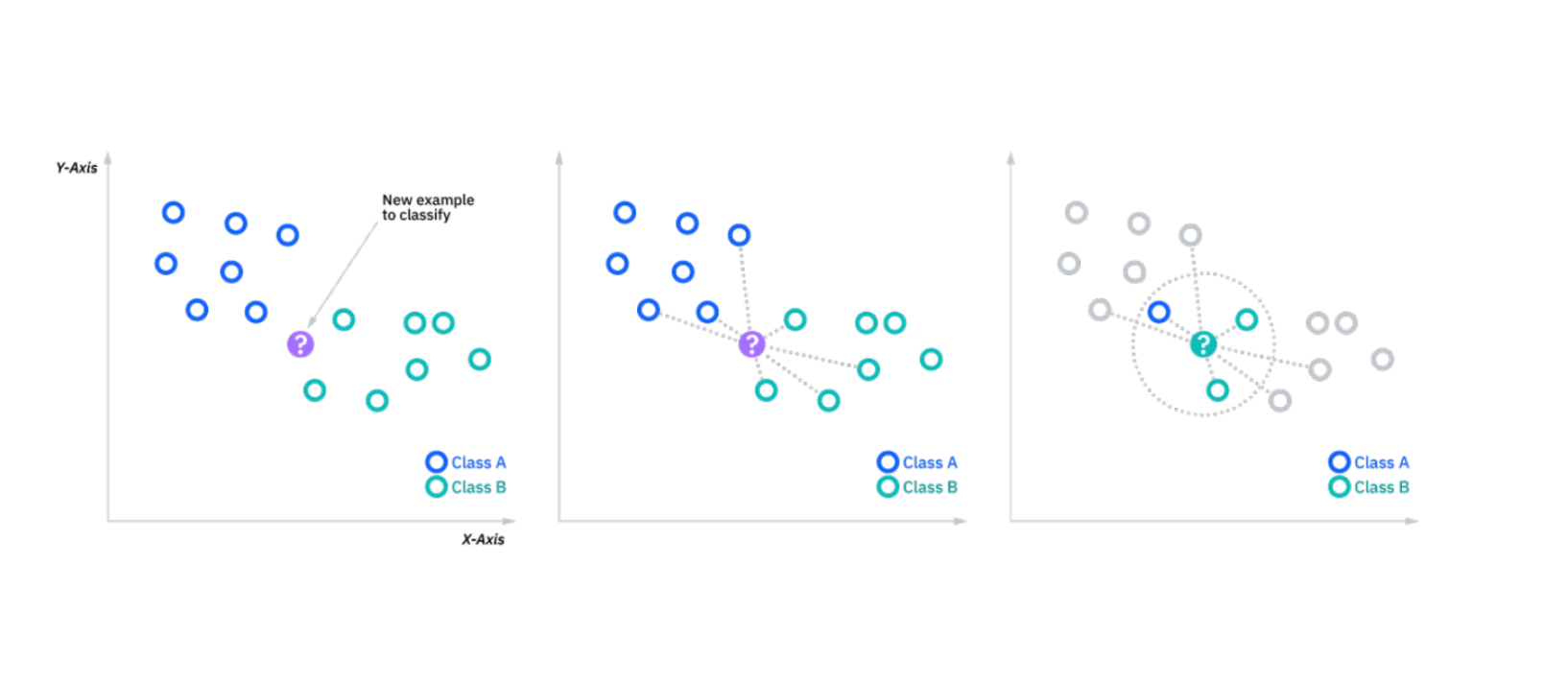 How KNN works between two classes. Source: https://www.ibm.com/in-en/topics/knn
Example of KNN in Action
A classic example of KNN in action is a recommendation system for a movie streaming service. Imagine a platform that uses the KNN algorithm to suggest movies to users based on their past viewing history and ratings. The algorithm identifies the K nearest neighbors to a given user, where the neighbors are other users with similar viewing habits. By analyzing the preferences of these neighbors, the system can recommend movies that are highly rated by them but not yet watched by the target user. This personalized recommendation approach not only enhances user experience but also increases user engagement and satisfaction, showcasing the practical power of the KNN algorithm.
Weighted KNN Variants
Standard KNN treats all neighbors equally, but this might not be ideal as closer neighbors should logically have more influence on predictions. Weighted KNN addresses this by assigning weights to neighbors based on their distance:
The weight of each neighbor is typically the inverse of its distance from the query point.
For classification, weighted voting is performed.
For regression, a weighted average is calculated.
The formula for a simple distance-weighted approach might look like:
weighti=1d(x,xi)2\text{weight}_i = \frac{1}{d(x, x_i)^2}weighti=d(x,xi)21
Where d(x, xi) is the distance between the query point x and the neighbor xi.
Optimizing KNN Performance
Cross-Validation Strategies for Finding Optimal k
K-fold cross-validation is commonly used to determine the optimal value of k. The process involves:
Splitting the dataset into k folds (not to be confused with the k in KNN).
For each value of k in KNN (e.g., k=1 to k=20):
Train and evaluate the model k times, each time using a different fold as the test set.
Calculate the average performance across all k folds.
Select the k value that gives the best average performance.
Elbow Method
The elbow method involves plotting the model's performance (e.g., accuracy or error rate) against different values of k and looking for an "elbow point" where the rate of improvement significantly decreases. This point often indicates a good trade-off between bias and variance.
Grid Search Implementation
Grid search is a systematic way to try different combinations of hyperparameters (including k and possibly similarity metrics) and select the combination that gives the best performance on a validation set.
Handling Class Imbalance
KNN can be sensitive to class imbalance, where some classes have many more examples than others. Strategies to address this include:
Resampling: Oversampling minority classes or undersampling majority classes.
Different evaluation metrics: Using metrics like F1-score or AUC instead of accuracy.
Weighted voting: Assigning different weights to classes based on their frequency.
Dimensionality Considerations and the Curse of Dimensionality
As the number of dimensions (features) increases, the volume of the space increases exponentially. This phenomenon, known as the "curse of dimensionality," can make distance metrics less meaningful and KNN less effective. In high-dimensional spaces:
Data points tend to be equidistant from each other.
The concept of "nearest" becomes less clear.
The model requires exponentially more data.
To combat this, consider:
Feature selection to remove irrelevant features
Dimensionality reduction techniques like PCA
Using specialized data structures like KD-trees for efficient nearest neighbor search
Practical Implementation
Let's implement KNN for a classification task using Python and scikit-learn.
Importing the modules
import numpy as np
import pandas as pd

import matplotlib.pyplot as plt

from sklearn.datasets import make_blobs
from sklearn.neighbors import KNeighborsClassifier
from sklearn.model_selection import train_test_split
from sklearn.metrics import accuracy_score
Dataset
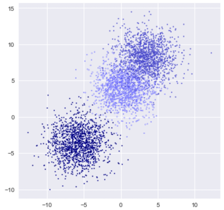
Scikit-learn can be used for training samples creating synthetic datasets, which are great for demo purpose.
X, y = make_blobs(n_samples = 4000, n_features = 3, centers = 3 ,cluster_std = 2, random_state = 80)
X
array([[ 7.60190561,  4.86336321,  6.97616573],
       [ 5.97809745,  7.69910922,  2.77419701],
       [-4.36024844, -2.23247572, -5.29113293],
       ...,
       [-8.22252297, -6.88609334, -6.52102135],
       [-3.96254707, -5.27559922, -2.70880022],
       [-4.25865881, -1.67791521, -3.70523373]])
y
array([1, 1, 2, ..., 2, 2, 2])
Plot
plt.figure(figsize = (6,6))
plt.scatter(X[:,0], X[:,1], c=y, marker= '.', s=10, edgecolors='blue')
plt.show()
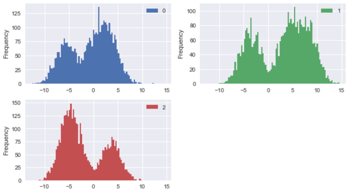
df = pd.DataFrame(X)
df.head()
plt.rcParams['figure.figsize']=(10,15)
df.plot(kind='hist', bins=100, subplots=True, layout=(5,2), sharex=False, sharey=False)
plt.show()
The K-Nearest Neighbors Classifier implementation
The first step is to figure out optimal value for the k. The calculation of the K value varies greatly depending on the situation. The default value of K when using the Scikit-Learn Library is 5 and the default distance metric used is Euclidean.
Tuning the Model to Get High K Nearest Neighbor Accuracy
from sklearn.model_selection import GridSearchCV
param_grid = {'n_neighbors':np.arange(1,4)}

knn = KNeighborsClassifier()
knn_cv= GridSearchCV(knn,param_grid,cv=5)
knn_cv.fit(X,y)

print(knn_cv.best_params_)
print(knn_cv.best_score_)
{'n_neighbors': 3}
0.9887499999999999
#train-test split
X_train, X_test, y_train, y_test = train_test_split(X, y, random_state = 80)
# instantiate the model
knn = KNeighborsClassifier(n_neighbors=3)

# fit the model to the training set
knn.fit(X_train, y_train)

y_pred = knn.predict(X_test)

print('Model accuracy score: {0:0.4f}'. format(accuracy_score(y_test, y_pred)))
Model accuracy score: 0.9890.
We got an accuracy rate of 98.90%, which is considered very good. We increased the number of neighbours from 1 to 4, and the model performed best at k=3.
The K Nearest Neighbor model does not involve any training period since the data itself is a model that will be the reference for future training phase prediction. As a result, it is time-efficient, enabling quick improvisation for random modeling on the available data.
KNN only requires two hyperparameters, a K value and a distance metric, making it simpler to tune than other machine learning algorithms.
Most classifier algorithms are easy to implement for binary classification problems but require extra effort to implement for multi-class problems. In contrast, KNN adapts to multi-class problems without any extra effort.
Main Mechanism
The main mechanism of the KNN algorithm involves identifying the K nearest neighbors to a given data point and using their class labels to make a prediction. For classification tasks, the algorithm assigns the class that is most common among the K nearest neighbors. For regression tasks, it averages the values of the K nearest neighbors to predict the value of the new data point. This approach is widely used in various domains due to its simplicity and effectiveness, allowing it to handle both classification and regression problems with ease.
Performance Metrics Evaluation
When evaluating KNN models, consider multiple metrics beyond just accuracy:
Accuracy: The proportion of correct predictions.
Precision: The proportion of positive identifications that were actually correct.
Recall: The proportion of actual positives that were identified correctly.
F1-score: The harmonic mean of precision and recall.
Confusion matrix: A table showing correct and incorrect classifications for each class.
ROC curve and AUC: For binary classification, showing the trade-off between true positive rate and false positive rate.
Tips for Scaling to Larger Datasets
KNN can become computationally expensive with large datasets. Here are some strategies to improve efficiency:
Use approximate nearest neighbor algorithms: Algorithms like locality-sensitive hashing (LSH) can find approximate nearest neighbors much faster than exact methods.
Implement KNN variants for efficiency: Data structures like KD-trees and ball trees organize the data to make nearest neighbor search more efficient:
KD-trees: Partition the space using hyperplanes, allowing for quick elimination of large portions of the search space.
Ball trees: Partition the space using hyperspheres, which can be more effective than KD-trees in high-dimensional spaces.
Sample the training data: For very large datasets, using a representative sample can significantly reduce computation time with minimal impact on accuracy.
Parallel processing: Utilize multi-core processors or distributed computing to speed up distance calculations.
Real-World Applications
KNN is widely used across various domains due to its simplicity and effectiveness:
Recommendation Systems
KNN is the basis for collaborative filtering in recommendation systems. By finding users with similar preferences (nearest neighbors), the system can recommend items that those similar users liked but the target user hasn't seen yet.
Case Study: Movie Recommendation
A streaming service might use KNN to recommend movies to users based on their viewing history. The algorithm would find users with similar viewing patterns and recommend movies that these similar users enjoyed but the target user hasn't watched yet.
Medical Diagnosis
KNN can help in medical diagnosis by finding patients with similar symptoms or test results and using their diagnoses to predict the diagnosis for a new patient.
Case Study: Diabetes Prediction
Using features like glucose level, BMI, age, and blood pressure, KNN can classify whether a patient is likely to have diabetes by comparing their metrics with those of patients with known diagnoses.
Image Recognition
In computer vision, KNN can be used for image classification by comparing feature vectors extracted from images.
Example Project: Handwritten Digit Recognition
Using the MNIST dataset, we can implement KNN to recognize handwritten digits. Each image is represented as a vector of pixel values, and the algorithm classifies new images based on similarity to training images.
Anomaly Detection
KNN can identify anomalies or outliers by finding points that are far from their nearest neighbors.
Implementation Example: Credit Card Fraud Detection
By calculating the average distance to the knn for each transaction, those with unusually large distances can be flagged as potential fraud.
Vector Similarity Search
In high-dimensional vector spaces like those used in NLP and computer vision, KNN can efficiently find similar items. This is particularly valuable in applications such as:
Image similarity search
Document clustering
Entity matching
For these applications, specialized vector databases can significantly improve performance compared to traditional databases, especially when dealing with high-dimensional data where calculating similarity is computationally intensive.
Limitations and Alternatives
When KNN Fails
Despite its simplicity and effectiveness, KNN has several limitations:
Computationally expensive: For large datasets, calculating distances between all pairs of points can be prohibitively expensive.
The curse of dimensionality: In high-dimensional spaces, the concept of distance becomes less meaningful, making KNN less effective.
Imbalanced data: KNN can be biased toward the majority class in imbalanced datasets.
Sensitive to noise and irrelevant features: Since KNN relies on distance calculations, noisy or irrelevant features can significantly impact its performance.
Memory intensive: KNN requires storing the entire training dataset in memory.
Advantages of KNN
Despite these limitations, KNN offers several advantages:
No training period: The KNN model does not involve any training period since the data itself is the model. This makes it time-efficient, enabling quick improvisation for random modeling on available data.
Simple hyperparameter tuning: KNN only requires two main hyperparameters—a k value and a similarity metric—making it simpler to tune than many other machine learning algorithms.
Natural multi-class support: Unlike many classifier algorithms that require extra effort to implement for multi-class problems, KNN adapts to multi-class problems without any additional complexity.
Non-parametric nature: KNN makes no assumptions about the underlying data distribution, allowing it to capture complex patterns that parametric models might miss.
Computational Complexity Considerations
Time complexity for prediction: O(MN log(k)) for each prediction, where M is the dimension of the data (number of features) and N is the size or number of instances in the training dataset. This is because:
Computing distances between the query point and all training points: O(MN)
Finding the knn (typically using a partial sort): O(N log(k))
Space complexity: O(MN) for storing the training dataset.
This computational complexity can make KNN impractical for large datasets without optimization. However, there are specialized data structures and algorithms that can make KNN more efficient even for large datasets.
Alternative Algorithms
When KNN isn't suitable, consider these alternatives:
Decision Trees and Random Forests: Better handle irrelevant features and can provide feature importance.
Support Vector Machines (SVM): More effective in high-dimensional spaces and with complex decision boundaries.
Naive Bayes: Computationally efficient and works well with high-dimensional data.
Neural Networks: Capable of learning complex patterns but require more data and computational resources.
Hybrid Approaches
Combining KNN with other algorithms can overcome some of its limitations:
KNN with feature selection/extraction: Apply feature selection techniques before using KNN to reduce dimensionality.
Ensemble methods: Combine KNN with other algorithms through voting or stacking.
Local weighted regression: Use KNN to identify local neighborhoods, then apply regression within each neighborhood.
Conclusion and Further Resources
K-Nearest Neighbors is a powerful and intuitive algorithm that leverages the simple concept that similar instances tend to have similar outcomes. Despite its simplicity, KNN can be highly effective when implemented correctly, with appropriate preprocessing, parameter selection, and optimization techniques.
Key Takeaways
KNN is a non-parametric, instance-based learning algorithm that can be used for both classification and regression tasks.
The choice of similarity metric and the value of k are crucial for KNN's performance.
Feature scaling is essential before applying KNN to ensure all features contribute equally to distance calculations.
KNN can suffer from the curse of dimensionality and can be computationally expensive for large datasets.
Efficient implementations using KD-trees or ball trees can significantly improve performance.
Future Directions for KNN Research
Despite its simplicity and effectiveness, the KNN algorithm has several limitations, such as sensitivity to noise and outliers, high computational cost, and the need for substantial memory to store the training data. Future research directions for KNN include developing more efficient algorithms to handle large datasets, improving robustness to noise and outliers, and exploring new similarity metrics and weighting schemes. Additionally, researchers are investigating the integration of KNN with emerging technologies like deep learning, natural language processing, and computer vision. By addressing these challenges and expanding its applications, the continued development of the KNN algorithm will significantly impact the field of data science, ensuring its relevance and utility in solving complex problems.
Academic Papers and Resources
For those interested in delving deeper into KNN and its variants, consider these resources:
Cover, T. M., & Hart, P. E. (1967). "Nearest neighbor pattern classification." IEEE Transactions on Information Theory, 13(1), 21-27.
Altman, N. S. (1992). "An introduction to kernel and nearest-neighbor nonparametric regression." The American Statistician, 46(3), 175-185.
Weinberger, K. Q., & Saul, L. K. (2009). "Distance metric learning for large margin nearest neighbor classification." Journal of Machine Learning Research, 10, 207-244.
Online Courses and Tutorials
Coursera: Machine Learning by Andrew Ng
Kaggle: Feature Engineering and KNN
scikit-learn Documentation: Nearest Neighbors
By thoroughly understanding the KNN algorithm, implementation details, and optimization techniques, you'll add a versatile and powerful tool to your machine learning toolkit that can be applied across numerous domains.
Keep Reading

Vector Lakebase: End the AI Data Silo
Learn how Vector Lakebase unifies vector search, data lakes, and AI data operations so teams can serve RAG and agents without copy-and-sync pipelines.

Zilliz Cloud Audit Logs Goes GA: Security, Compliance, and Transparency at Scale
Zilliz Cloud Audit Logs are now GA, giving enterprises real-time visibility, compliance-ready trails, and stronger security across AWS, GCP, and Azure.

Legal Document Analysis: Harnessing Zilliz Cloud's Semantic Search and RAG for Legal Insights
Enhance legal document analysis with Zilliz Cloud’s Semantic Search and RAG. Improve accuracy, efficiency, and scalability for contracts, case law, and compliance.