Enhancing Efficiency in Vector Searches with Binary Quantization and Milvus
Binary quantization represents a transformative approach to managing and searching vector data within Milvus, offering significant enhancements in both performance and efficiency. By simplifying vector representations into binary codes, this method leverages the speed of bitwise operations, substantially accelerating search operations and reducing computational overhead.
Read the entire series
- Raft or not? The Best Solution to Data Consistency in Cloud-native Databases
- Understanding Faiss (Facebook AI Similarity Search)
- Information Retrieval Metrics
- Advanced Querying Techniques in Vector Databases
- Popular Machine-learning Algorithms Behind Vector Searches
- Hybrid Search: Combining Text and Image for Enhanced Search Capabilities
- Ensuring High Availability of Vector Databases
- Ranking Models: What Are They and When to Use Them?
- Navigating the Nuances of Lexical and Semantic Search with Zilliz
- Enhancing Efficiency in Vector Searches with Binary Quantization and Milvus
- Model Providers: Open Source vs. Closed-Source
- Embedding and Querying Multilingual Languages with Milvus
- An Ultimate Guide to Vectorizing and Querying Structured Data
- Understanding HNSWlib: A Graph-based Library for Fast Approximate Nearest Neighbor Search
- What is ScaNN (Scalable Nearest Neighbors)?
- Getting Started with ScaNN
- Next-Gen Retrieval: How Cross-Encoders and Sparse Matrix Factorization Redefine k-NN Search
- What is Voyager?
- What is Annoy?
Introduction
In today's data-driven world, we value efficiency in dealing with and searching through massive datasets, especially when it comes to high-dimensional vector data. A method that has come to the rescue is binary quantization. It simplifies the storage and manipulation of vectors by reducing every element to a binary digit, either 0 or 1. Reducing the complexity and size of data enhances processing speeds and improves storage efficiency.
Milvus is a scalable vector database specifically designed to facilitate efficient similarity searches within large-scale vector datasets. While Milvus does not currently support binary quantization, it remains highly effective at storing and utilizing pre-quantized binary vectors through its efficient binary indexes. This indexing capability significantly enhances the performance of similarity searches within large-scale datasets of vectors. By using binary indexes, Milvus leverages faster bitwise operations during searches, which are computationally less intensive than operations required for floating-point vectors. As a result, Milvus can perform searches more rapidly and efficiently, which is particularly beneficial in environments handling massive datasets where quick response times are critical.
 Source: Dalle
Vector Databases and Embeddings
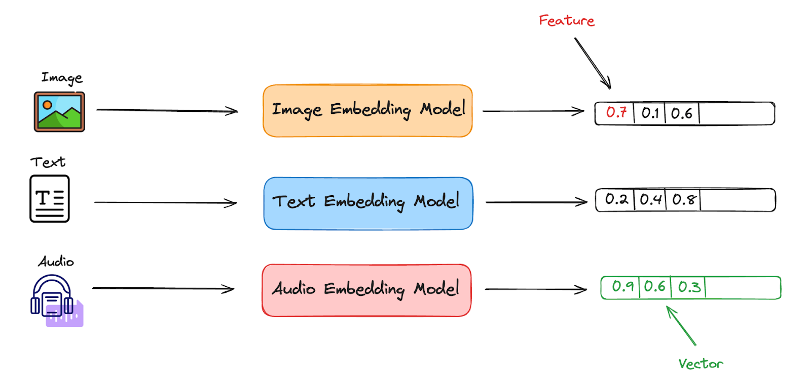
Before reviewing Binary Quantization, let’s briefly explain vector embeddings. Take, for example, the diagram below, which has three different data types: Images, Text, and Audio. These models transform each data point into an easily stored format, in this case, a vector/embedding. It does this by dividing the single data point into multiple features and giving each feature a given value. A vector database’s main goal is to handle vector embeddings generated by machine learning models.
 Image By Author
As you might imagine, a wide variety of vector embeddings can be stored within a vector database, each tailored for different types of data and analytical tasks.
Binary Embeddings
One of the main focuses of this article, Binary embeddings represent data as binary vectors, where each element of the vector is either 0 or 1. This type of embedding is particularly useful for tasks that require high efficiency in both storage and computational speed. Binary embeddings are often used in information retrieval systems where the simplicity of the data format allows for rapid similarity calculations.
Dense Embeddings
Dense embeddings represent data with vectors where each dimension contains a continuous value, typically derived from deep learning models. These embeddings capture a significant amount of information in a compact form, making them highly effective for tasks involving natural language processing, image recognition, and more. Dense embeddings are called so because the vectors generally have non-zero values in most dimensions, thereby carrying a rich set of information in each element.
Sparse Embeddings
Sparse embeddings, in contrast to dense embeddings, are characterized by vectors that contain a high number of zero values. These embeddings are efficient in representing data that is inherently dimensional but mostly empty or irrelevant. Sparse embeddings are useful in environments where only a few attributes are significant, such as in certain types of natural language data or user-item interaction data in recommender systems. This sparsity leads to more efficient storage and processing, especially when the system can skip over the zero values.
What is Binary Quantization?
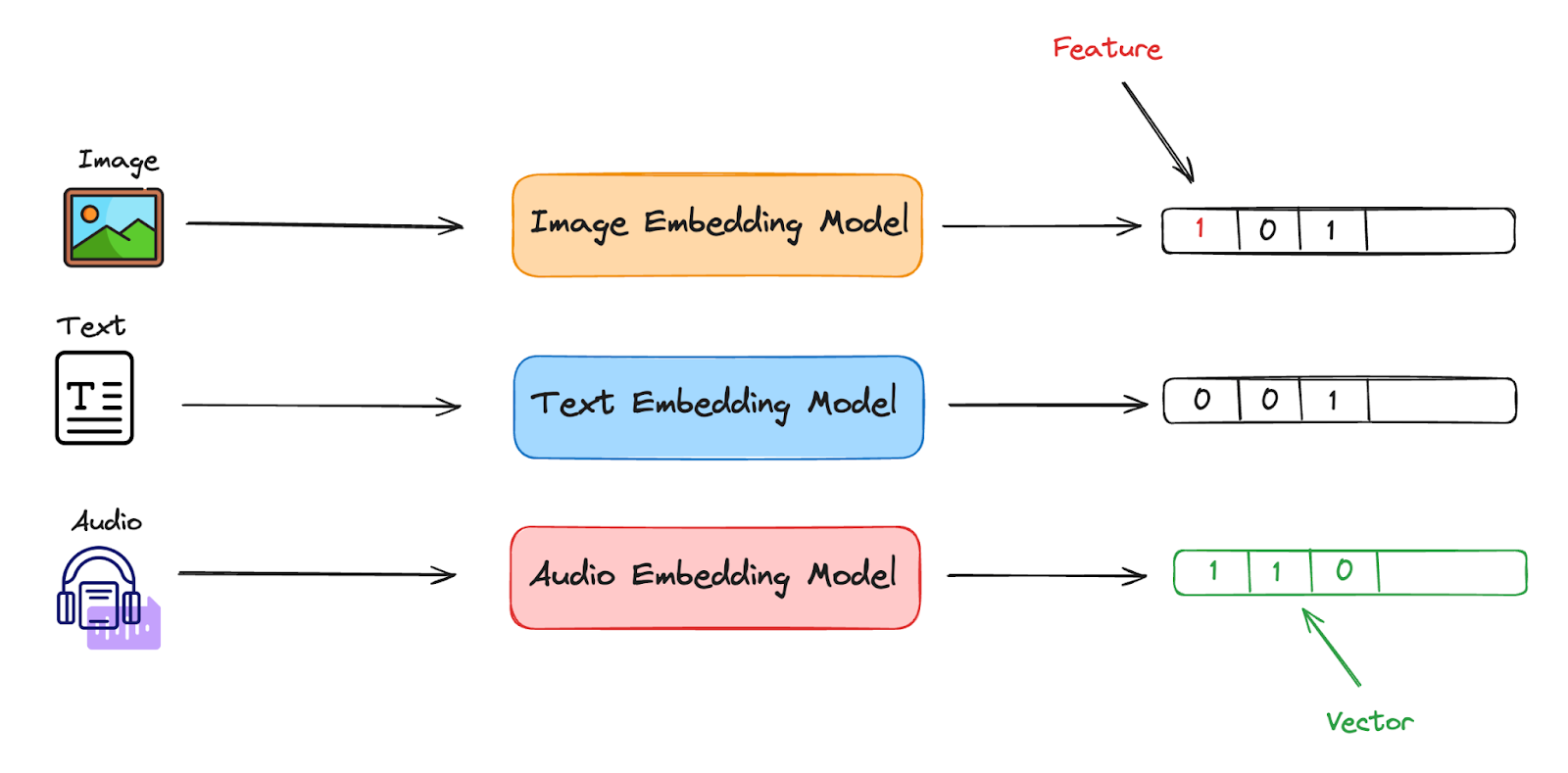
After the initial embedding is provided this is where Binary Quantization comes in handy. To put it simply, Binary quantization involves reducing each feature of a given vector(embedding) into a binary digit.
For example, if an image is represented by three distinct features, where each feature holds a value in the range of a FLOAT-32 storage unit, performing binary quantization on this vector would result in each of the three features being independently represented by a single binary digit. Thus, after binary quantization, the vector that originally contained three FLOAT-32 values would be transformed into a vector of three binary digits, such as [1, 0, 1].
 Image By Author
Now that you have an understanding of binary quantization, let's explore the advantages and disadvantages of this approach. While one clear con to such a process is the loss of precision, when it comes to vector database and retrieval systems, binary codes facilitate faster data indexing and searching.
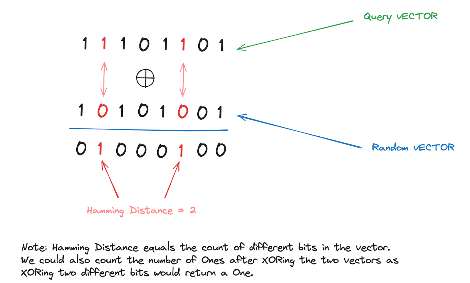
For example, using the Hamming Distance Calculations we can utilize the similarity between binary vectors in a quick and efficient manner, in which the Hamming process in this case requires simply just the count of differing bits. Such a calculation is much faster and less computationally intensive than measuring distances in floating-point space, which helps mitigate the drawback of some loss in the model’s precision.
The challenge with exact nearest neighbor searches in high-dimensional spaces is that they suffer from the "curse of dimensionality". As the dimensionality of data increases, the volume of the space increases exponentially, making it increasingly difficult to differentiate between distances in a meaningful way. This can lead to significant increases in computational and memory requirements.
The Advantages of Binary Quantization
Speed Enhancement
Binary Quantization offers high performance when conducting vector searches on massive datasets. Why is that? Simply put, because of the smaller and less complex computations. In the case of Milvus and binary vectors, Milvus utilizes the similarity metric known as the Hamming Distance. This metric can be used to calculate the distance between two stored binary vectors in negligible time. Below is an example of how the Hamming Distance method works.
 Image By Author
Storage Reduction and Data Efficiency
 Storage Reduction and Data Efficiency
By converting to binary, the storage requirement for this vector is reduced from 96 bits to just 3 bits. This is a substantial decrease, effectively reducing the storage size by over 31 times. Such reduction scales up significantly when applied across large datasets, leading to major savings in storage space and associated costs, while also enhancing processing speeds due to the simpler data format. This efficiency is especially beneficial in environments handling vast amounts of data, such as vector databases and large-scale analytical operations.
Implementing Binary Embeddings in Milvus
1) Preparation
This initial step is fundamental and aligns with standard data engineering practices. Initially, we will clean the data by eliminating any corrupt or outlier data points that could distort our analysis.
Next, we will engage in the process of feature selection to identify the most relevant features. This helps in reducing dimensionality and enhancing the efficiency of binary quantization.
Moving on, we can perform normalization, which is scaling the data to have a uniform range, typically [0,1] or mean zero and unit variance. This is important because it ensures that no single feature dominates due to its scale.
While the quantization process can still function without these preliminary steps, it becomes easier and more efficient when they are correctly performed.
2) Vector Transformation
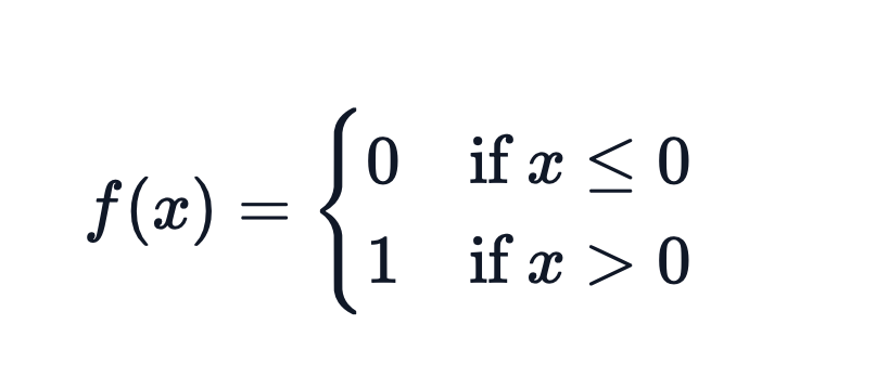
First, we will determine a threshold(x) for each dimension of the vector. Values in the vector that are above this threshold will be set to 1, while those below it will be set to 0.

To perform binary quantization manually you can use the following code with a threshold of 0.5:
| import numpy as np# Example datadata = np.array([0.85, 0.23, 0.76])# Setting a thresholdthreshold = 0.5# Binary quantizationbinary_data = np.where(data >= threshold, 1, 0)print(binary_data) |
To select a suitable threshold for each dimension of the vector, common methods involve using the median(middle value) or mean(average) of each feature across the dataset.
It’s essential to ensure that the chosen threshold maintains the integrity of the data’s structure, minimizing the loss of information.
3) Indexing with Milvus
Once your vectors are in binary, you can use Milvus to index them for efficient retrieval.
Before utilizing the search feature of Milvus, we must declare an index type along with the similarity search metric. For those of you who do not know what the index type represents, indexes are specialized data structures that help optimize the performance of queries.
Binary Index Types
Having said that, we would start by choosing our Index Type. For binary vectors, Milvus supports several index types such as BIN_FLAT and BIN_IVF_FLAT.
BIN_FLAT which are suitable for brute-force searching on binary data, while BIN_IVF_FLAT is an inverted file index that can help improve the efficiency on larger datasets.
In the case of utilizing BIN_IVF_FLAT, we will need to specify other metrics such as the number of clusters (nlist) which can affect both the accuracy and speed of the search.
4) Querying
Finally, querying binary vectors in Milvus involves setting up and executing searches based on similarity or matching. The below provided code will mainly focus on specifying our index type and metric, utilizing the BIN_FLAT index as our chosen type, along with the Hamming Distance as our similarity metric for the search. For more on the given steps, please check the following Milvus documentation.
Step 1: Connecting To Our Milvus Instance
Before proceeding with this step, ensure that you have created your own Milvus instance. Once that is set up, use the URI of your server to establish a connection by entering it into the MilvusClient() method.
| from pymilvus import MilvusClient# 1. Set up a Milvus clientclient = MilvusClient( uri="http://localhost:19530") |
Step 2: Configure Our Vector DB Schema, Search Index, and Metric
Creating our schema and adding new fields to it.
| schema = milvus_client.create_schema(enable_dynamic_field=True)schema.add_field("id", DataType.INT64, is_primary=True)schema.add_field("vector", DataType.BINARY_VECTOR, dim=dim)schema.add_field("city", DataType.VARCHAR, max_length=64) |
Preparing our index parameters.
| index_params = client.prepare_index_params() |
Adding indexes.
This section outlines the setting of Binary Quantization within our vector database. Here, we will configure the index type and set the metric type accordingly. This setup enables our schema to store data in binary format and utilize the Hamming Distance method to calculate the distances between vectors.
| index_params.add_index(field_name="my_id",metric_type="HAMMING",index_type="BIN_FLAT",params={"nlist": 1024}) |
Lastly, we will create the final collection using the configured index params. To know more about the schema parameter below please check the milvus documentation.
| client.create_collection( collection_name="cities", schema=schema, index_params=index_params) |
Step 3: Inserting Data To Our Vector Database
Following the documentation example, we will be inserting randomly generated vectors into our newly created DB.
| city = ["paris", “New York”, “Cairo”, “Tokyo”]data = [ {"id": i, "vector": [ random.uniform(-0, 1) for _ in range(5) ], "city": f"{random.choice(city)}_{str(random.randint(1, 5))}" } for i in range(5) ]res = client.insert( collection_name="cities", data=data) |
Step 4: Performing Binary Single Vector Search
Next, we will conduct the search. Initially, we will submit a specific vector as our query. Since we are using binary vectors, the Milvus database will convert the provided vector into its binary form. Subsequently, it will calculate the Hamming distance for each pre-stored vector, continuing this process until it identifies the vector that matches most closely.
| # Single vector searchres = client.search( collection_name="cities", # Replace with the actual name of your collection # Replace with your query vector binary_vectors = [] data=binary_vectors.append(bytes(np.packbits([0,1,1,0,0,1], axis=-1).tolist())) limit=1, # Max. number of search results to return search_params={"metric_type": "HAMMING", "params": {}} # Search parameters)# Convert the output to a formatted JSON stringresult = json.dumps(res, indent=4)print(result) |
Output
| [ [ { "id": 2, "distance": 1, "entity": {} } ]] |
The above result returns the most similar index in my vector database, along with the hamming distance of the vector to my original vector query.
Benchmark Analysis and Usage Recommendations
While binary quantization enhances search speeds by simplifying data computations, it can compromise accuracy, as binary codes may not capture the full nuances of the original data. This often leads to Recall Degradation, where the system's ability to retrieve all relevant vectors is reduced, affecting the recall rate.
Finding the optimal Speed-Accuracy balance is challenging, but users should define clear benchmarks for acceptable speed and accuracy to determine if a configuration meets their needs. The importance of this balance depends on the specific use of the vector database. In some scenarios, even minor accuracy losses are unacceptable, while in others, slight data deviations may not significantly impact outcomes.
Conclusion
Binary quantization represents a transformative approach to managing and searching vector data within Milvus, offering significant enhancements in both performance and efficiency. By simplifying vector representations into binary codes, this method leverages the speed of bitwise operations, substantially accelerating search operations and reducing computational overhead.
These improvements are crucial for applications dealing with large datasets and demanding real-time response capabilities. Therefore, if your application requires handling extensive data or demands quick data retrieval, consider exploring the binary quantization feature in Milvus.
Future Directions
As binary quantization continues to develop within the context of vector databases like Milvus, we can expect numerous advancements and innovations that will further refine and enhance vector search tasks. One such enhancement involves refining the process for setting appropriate thresholds for binary quantization. Furthermore, we anticipate the implementation of more sophisticated machine learning algorithms that can automatically adjust and optimize these thresholds based on real-time data analysis and feedback loops. This will not only improve the accuracy of the binary representations but also enhance the overall efficiency of search operations.
- Introduction
- Vector Databases and Embeddings
- What is Binary Quantization?
- The Advantages of Binary Quantization
- Implementing Binary Embeddings in Milvus
- Benchmark Analysis and Usage Recommendations
- Conclusion
- Future Directions
Content
Start Free, Scale Easily
Try the fully-managed vector database built for your GenAI applications.
Try Zilliz Cloud for FreeKeep Reading

Raft or not? The Best Solution to Data Consistency in Cloud-native Databases
Explain why consensus-based algorithms like Paxos and Raft are not the silver bullet and propose a solution to consensus-based replication.

Understanding HNSWlib: A Graph-based Library for Fast Approximate Nearest Neighbor Search
HNSWlib is an open-source C++ and Python library implementation of the HNSW algorithm, which is used for fast approximate nearest neighbor search.

What is Annoy?
Annoy is a lightweight, open-source library designed for fast, approximate nearest-neighbor searches in high-dimensional vector spaces.
