Learn
Retrieval Augmented Generation (RAG) 101

Pandas DataFrame: Chunking and Vectorizing with Milvus

Apr 25, 202416 min read

If we store all of the data, including the chunk text and the embedding, inside of Pandas DataFrame, we can easily integrate and import them into the Milvus vector database.

By Ruben Winastwan

Read the entire series

If we store all of the data, including the chunk text and the embedding, inside of a Pandas DataFrame, we can easily integrate and import them into the Milvus vector database.

Chunking or text splitting is a data preprocessing step of breaking down long texts into several smaller fragments called "chunks". This method becomes more and more relevant in today’s world if we want to fully leverage the powerful performance of LLMs or perform various custom analytics solutions with text data.

In this article, we’ll jump into the concept of chunking and its full meaning and importance in Natural Language Processing (NLP) and show you some examples of different methods to create chunks.

The Importance of Chunking

When dealing with NLP projects, our data normally comes in the form of raw texts. These raw texts could represent a sentence, a paragraph, or even a section of a book.

If our text data only represents short sentences, then chunking won’t be necessary. However, when our text data represents individual sentences, multiple sentences, or several paragraphs or a section of a book, chunking is an important step that we need to do. There are a couple of reasons for this.

Machine Learning Models Have a Maximum Token Length

Machine learning models can’t make sense of raw texts, and thus, we need to turn them into a format that can be understood by the model.

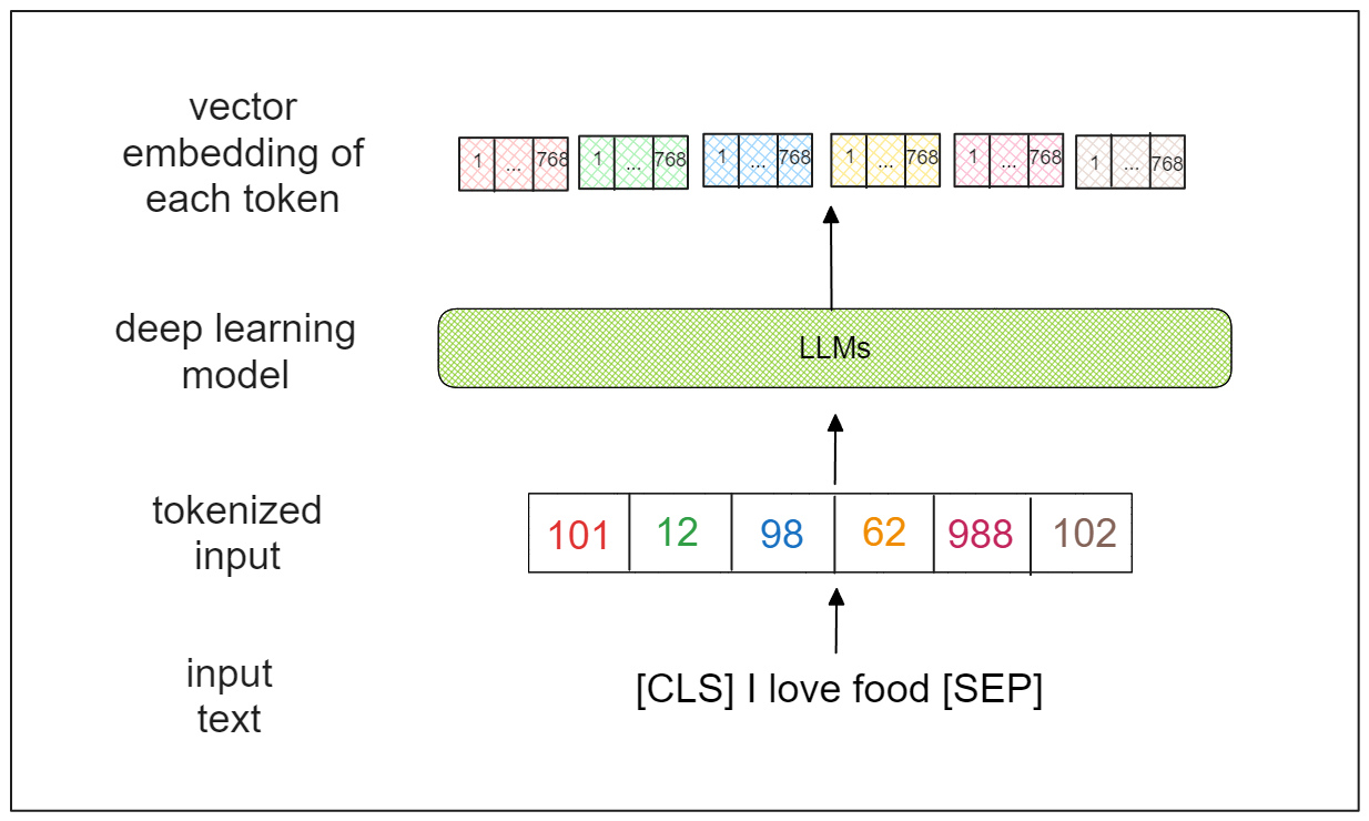
The standard way to do this is by transforming these raw texts into their numerical representation through a process called tokenization. An input text will be tokenized into a sequence of tokens and then transformed into each token’s integer mapping.

Image by author

The problem is that deep learning models have a certain limit of token length that they can handle. For example, BERT can take a maximum token length of 512. If the sequence of tokens is longer than that, BERT will automatically truncate our sequence, and this is something that we don’t want.

By chunking text into smaller segments, we can ensure that the tokenized input is still within the limit of the maximum token length of deep learning models.

For Information Retrieval

Let’s imagine a use case where one text data represents a whole book. If we have a query and want to fetch the most relevant content from the book, we need to find a way to effectively retrieve information from it.

One way to do this is by doing data segmentation, i.e splitting the text to produce chunks. Each chunk can represent a individual sentences, a paragraph, or even a section. The finer the granularity of the text splitting is, the more specific the information that we get.

Also, text and chunking strategy would be beneficial in an RAG scenario. If we manage to find the desired chunk size, we could get highly relevant context that helps LLMs to generate more accurate responses.

The problem is, text chunking is quite tricky to fine-tune especially for context preservation. When we chunk our text data into a very granular level, we run the risk of getting information that’s not really meaningful. On the other hand, if we chunk our data into a very broad level, we might get information that’s not really specific. Therefore, it’s important for us to understand the nature of our data before applying the chunking methods.

Chunking Methods

There are two commonly applied chunking techniques to create chunks: fixed-size chunking and content-aware chunking. We’re going to discuss each technique one at a time.

Fixed-Size Chunking

Fixed-size chunking refers to the process of splitting a text into smaller chunks, of a fixed and equal size. This means that you set a predefined chunk size in advance, and each chunk of the text will then have the same size as the predefined value.

Optionally, we can also define an overlap value. The overlap acts as a buffer to ensure that the semantic meaning of a text doesn’t get lost between two smaller chunks.

This technique is the simplest to implement and not as computationally expensive as the other upcoming techniques.

Now let’s implement this technique. Let’s consider the following text that talks about basketball.

text_input= """
Basketball is a team sport in which two teams, most commonly of five players each, opposing one another on a rectangular court, compete with the primary objective of shooting a basketball (approximately 9.4 inches (24 cm) in diameter) through the defender's hoop (a basket 18 inches (46 cm) in diameter mounted 10 feet (3.048 m) high to a backboard at each end of the court), while preventing the opposing team from shooting through their own hoop. A field goal is worth two points, unless made from behind the three-point line, when it is worth three. After a foul, timed play stops and the player fouled or designated to shoot a technical foul is given one, two or three one-point free throws. The team with the most points at the end of the game wins, but if regulation play expires with the score tied, an additional period of play (overtime) is mandated.

Players advance the ball by bouncing it while walking or running (dribbling) or by passing it to a teammate, both of which require considerable skill. On offense, players may use a variety of shots - the layup, the jump shot, or a dunk; on defense, they may steal the ball from a dribbler, intercept passes, or block shots; either offense or defense may collect a rebound, that is, a missed shot that bounces from rim or backboard. It is a violation to lift or drag one's pivot foot without dribbling the ball, to carry it, or to hold the ball with both hands and then resume dribbling.
"""

To illustrate a fixed-size chunking technique, we’re going to split this basketball text into three different sizes of chunks: 50 characters, 250 characters, and 1000 characters.

There are several options to chunk our data character-wise, as there are many Python data processing libraries that you can use out there. However, we’ll use LangChain in this demonstration.

from langchain_text_splitters import CharacterTextSplitter

for n in [50, 250, 500]:
    print(f"-------------------------------")
    text_splitter = CharacterTextSplitter(
        chunk_size = n,
        separator="",
        chunk_overlap=0,
        length_function=len,
        is_separator_regex=False,
    )
    chunk_text = text_splitter.split_text(text_input)
    for i in range(3):
      print(f"chunk {i}: {chunk_text[i]}")
  
"""
-------------------------------
chunk 0: Basketball is a team sport in which two teams, mo
chunk 1: st commonly of five players each, opposing one ano
-------------------------------
chunk 0: Basketball is a team sport in which two teams, most commonly of five players each, opposing one another on a rectangular court, compete with the primary objective of shooting a basketball (approximately 9.4 inches (24 cm) in diameter) through the de
chunk 1: fender's hoop (a basket 18 inches (46 cm) in diameter mounted 10 feet (3.048 m) high to a backboard at each end of the court), while preventing the opposing team from shooting through their own hoop. A field goal is worth two points, unless made from
-------------------------------
chunk 0: Basketball is a team sport in which two teams, most commonly of five players each, opposing one another on a rectangular court, compete with the primary objective of shooting a basketball (approximately 9.4 inches (24 cm) in diameter) through the defender's hoop (a basket 18 inches (46 cm) in diameter mounted 10 feet (3.048 m) high to a backboard at each end of the court), while preventing the opposing team from shooting through their own hoop. A field goal is worth two points, unless made from
chunk 1: behind the three-point line, when it is worth three. After a foul, timed play stops and the player fouled or designated to shoot a technical foul is given one, two or three one-point free throws. The team with the most points at the end of the game wins, but if regulation play expires with the score tied, an additional period of play (overtime) is mandated.

Players advance the ball by bouncing it while walking or running (dribbling) or by passing it to a teammate, both of which require conside
"""

We can observe the effects of different chunk lengths from the text chunking output above:

50 characters: The information for the smaller chunks is very granular, and extracting meaningful information from the chunk is challenging.
250 characters: Provides more or less sufficient information in each chunk.
500 characters: Offers elaborated information in one chunk. However, there's a higher risk of obtaining noisy information that isn't relevant to the context.

In general, information contained in text with a small chunk size is too granular to extract meaningful insights, while text with a large chunk size tends to be overly broad, making it difficult to extract specific information.

Content-Aware Chunking

Content-Aware chunking employs a more flexible approach to chunk size. Unlike fixed-size, chunking methods, the chunk size here is more of an output rather than an input parameter. The chunk size may vary for each split text depending on the context implemented.

A simple approach is to split the text based on whitespace or markers such as commas, periods, colons, semicolons, etc. Depending on the input type, text splitting can also be based on HTML sections or Markdown subheadings.

Now let’s implement text splitting based on the whitespace of our text:

text_splitter = CharacterTextSplitter(
        chunk_size = 25,
        separator=" ",
        chunk_overlap=0,
        length_function=len,
        is_separator_regex=False,
    )
chunk_text = text_splitter.split_text(text_input)
print(chunk_text[0])
"""
Output:
Basketball is a team
"""

In the above code, we've implemented text splitting based on whitespace, with each chunk containing approximately 25 characters. However, now the text splits between whitespace, ensuring that no words adjacent sentences are cut in the middle, unlike in the previous fixed-size chunking method.

Another more advanced text processing method is the recursive method. This approach divides texts into smaller segments in a hierarchical manner. Initially, we define the minimum chunk size. Then, it attempts to split the text at the broadest level, such as at a paragraph-level. If the splitting at the paragraph-level doesn't meet the minimum chunk size, it further splits the text at a sentence-level, then at a whitespace-level, and finally at a character-level.

In addition to text structure, we can also split text based on the embedding models we intend to use. As mentioned in the previous section, all deep learning models have specific token chunk lengths they can handle. If we aim to use a model from Sentence Transformers as an embedding model, we can adjust the chunk size to match the token length suitable for that model. Here’s how we can implement this with LangChain.

from langchain_text_splitters import SentenceTransformersTokenTextSplitter

splitter = SentenceTransformersTokenTextSplitter(chunk_overlap=0, model_name='sentence-transformers/all-mpnet-base-v2')
text_chunks = splitter.split_text(text=text_to_split)

Text Chunking Implementation

Now that we've explored different chunking techniques, let’s move on to the implementation. If you’d like to follow along, you can refer to the following notebook.

The data we'll be using is a large text dataset sourced from Wikipedia and is available for download on the HuggingFace dataset. While there are hundreds of thousands of texts available, for writing this demonstration, we'll focus on one that discusses basketball.

!pip install datasets

import pymilvus
import pandas as pd
from pymilvus import MilvusClient
from pymilvus import (
   utility,
   FieldSchema, CollectionSchema, DataType,
   Collection, AnnSearchRequest, RRFRanker, connections,
)
from langchain_text_splitters import CharacterTextSplitter
from datasets import load_dataset, Dataset

dataset = load_dataset(
    "wikimedia/wikipedia", "20231101.en", split="train", streaming=True
)

data = Dataset.from_dict({})
for i, entry in enumerate(dataset):
    # each entry has the following columns
    # ['id', 'url', 'title', 'text']
    if entry["title"] =="Basketball":
      data = data.add_item(entry)
    if i == 30000:
        break
# free memory
del dataset

You can experiment with any chunking strategy mentioned in the previous section, but we’re going to implement a content-aware chunking method, where one chunk represents one paragraph. To do so, we need to use “n” as the separator argument of the CharacterTextSplitter()class from LangChain.

text_splitter = CharacterTextSplitter(
    separator="\\n",
    chunk_size = 10,
    chunk_overlap=0,
    length_function=len,
    is_separator_regex=False,
)

chunk_text = [text_splitter.split_text(text) for text in data["text"]][0]
print(len(chunk_text))
"""
Output: 196
"""

As you can see from the illustration above, now each chunk represents topic sentence or a paragraph. After the chunking process, now we have in total 196 chunks. Let’s put only chunk ID and text chunk inside of Pandas to enforce the DataFame optimization.

df = pd.DataFrame()
df["chunk_id"] = [i for i in range(len(chunk_text))]
df["text_chunk"] = chunk_text

Text Vectorization

Now that we've split our text into chunks, the next step is to convert each chunk into embeddings.

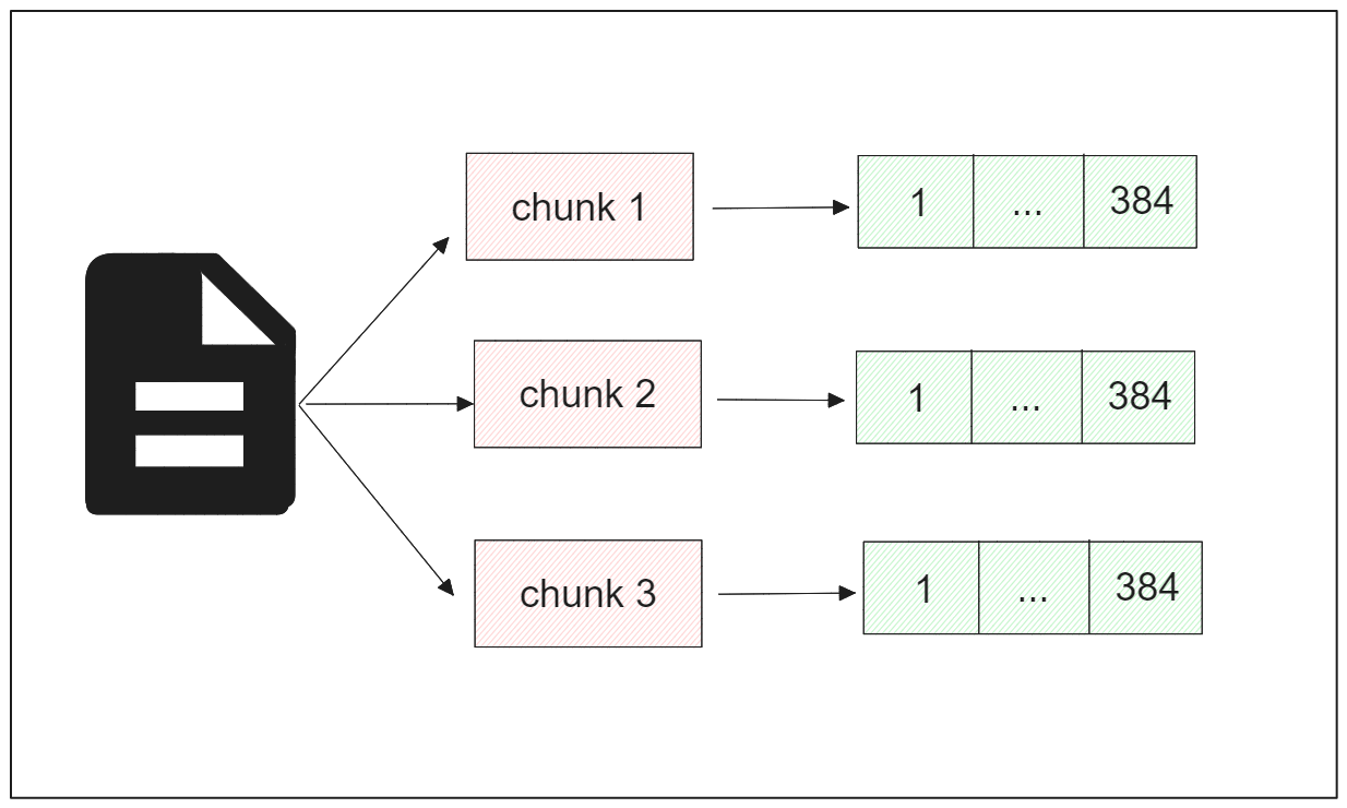
An embedding is a numerical representation of text, consisting of a vector of a particular dimension. Depending on the model used, there are two types of vector embeddings: dense vectors and sparse vectors.

A dense vector is typically generated by deep learning models such as those from OpenAI or Sentence Transformers. It contains rich information about the text it represents in a compact form, hence the name "dense."

On the other hand, a sparse vector usually has higher dimensionality than a dense vector, with most of its values being zero. This vector is often generated by models that use a bag-of-words method like BM25. In more recent advancements, a learned sparse vector via a model called SPLADE has been introduced to add more contextual information to the sparse vector.

Image by author

After converting the chunks into embeddings, we can later perform text analytics, semantic analysis, and vector search on them.

For this demonstration, we'll utilize the all-MiniLM-L6-v2 model from Sentence Transformers to convert chunks into dense embeddings. This model generates an embedding for each chunk with a dimension of 384.

Integrating a Sentence Transformer model with Milvus is straightforward. We simply need to call the SentenceTransformerEmbeddingFunction class from Milvus and specify the name of the model we want to use. For the list of available models from Sentence Transformers, refer to their documentation.

from pymilvus import model

sentence_transformer_ef = model.dense.SentenceTransformerEmbeddingFunction(
    model_name='all-MiniLM-L6-v2', # Specify the model name
    device='cpu' # Specify the device to use, e.g., 'cpu' or 'cuda:0'
)

To convert each chunk into an embedding, we can use the encode_documents() method.

chunk_text = df["text_chunk"].values.tolist()
chunk_embeddings = sentence_transformer_ef.encode_documents(chunk_text)
df["chunk_embeddings"] = chunk_embeddings

print(chunk_embeddings[0])
"""
Output
[ 3.87127437e-02  6.21908298e-03 -2.17081346e-02 -7.02043846e-02
  4.95888777e-02  2.59143058e-02  3.53455357e-02 -1.74768399e-02
  .............................................................
  .............................................................
   -2.22174134e-02  2.56354176e-02  3.62051129e-02 -7.05866441e-02
  2.83311424e-03  6.06332906e-02  2.30652522e-02 -2.65785996e-02]
  """

And there we have it. Now we can import all of the chunks as well as the embeddings into a vector database, and we’re going to use Milvus for that.

Milvus Database Integration and Semantic Search

What we have now is essentially a Pandas DataFrame with the text, ID, and embedding of each chunk as columns. If our data is organized in a Pandas DataFrame, we can easily import it into a Milvus database with a simple method.

Using the construct_from_dataframe() method from the Collection class, the data within the Pandas DataFrame can be imported into the database. All we need to do is specify the name of the collection, the primary field, and provide the DataFrame itself.

connections.connect("default", host="localhost", port="19530")

col, results = Collection.construct_from_dataframe(
    name="chunk_demo",
    primary_field="chunk_id",
    dataframe=df,
)
dense_index = {"index_type": "FLAT", "metric_type": "COSINE"}
col.create_index("chunk_embeddings", dense_index)
col.flush()

In the code above, we also create an index for the chunk embeddings to facilitate fast and easy retrieval during a vector search. The distance metric used for semantic similarity search later on is cosine similarity.

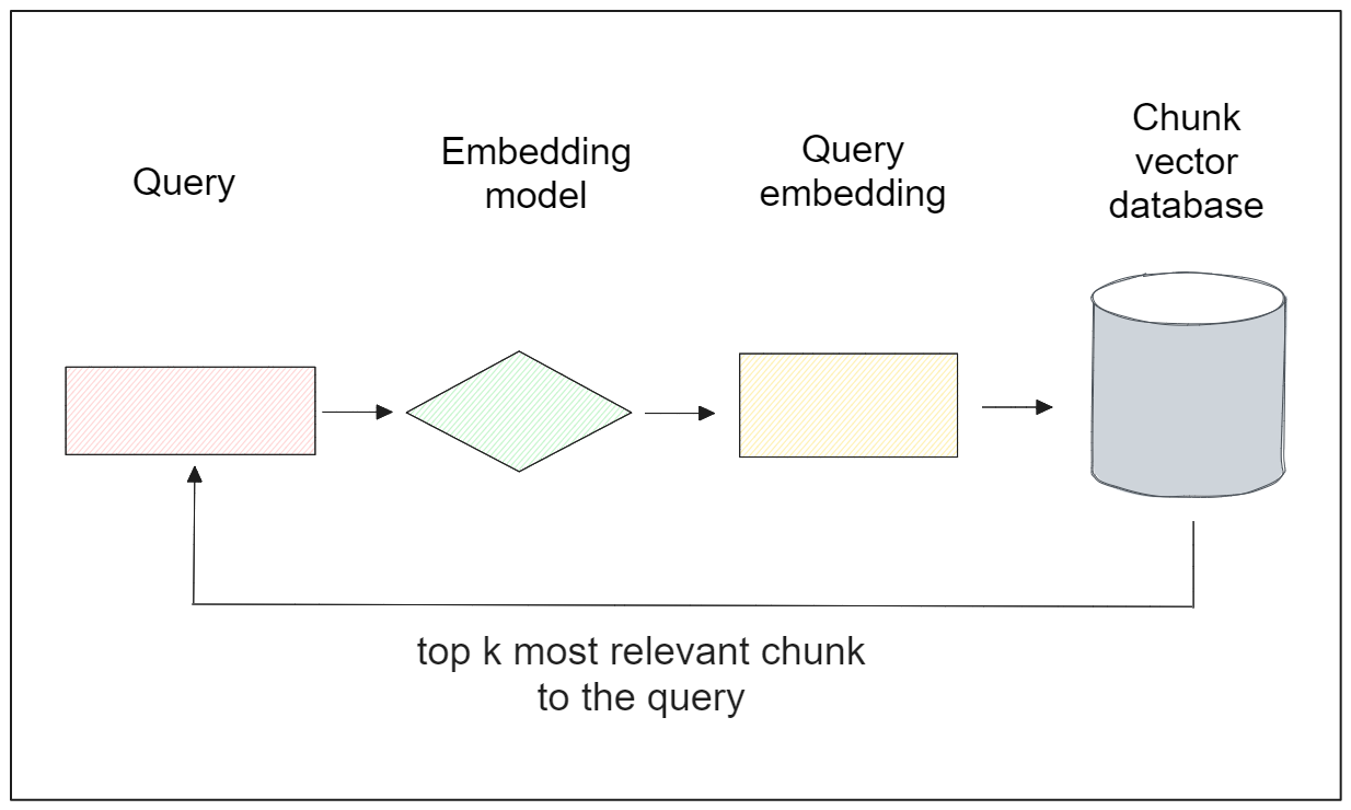
Now that we've imported the data into the database, we can perform various tasks with it. Among others, semantic similarity is the most popular. In this task, the most similar item in the database will be retrieved based on a specific query, as illustrated in the visualization below:

Let’s say we have the following query: "Who are some of the greatest players in the history of basketball?" and we want to retrieve the relevant paragraph that addresses this query. To achieve this, the query needs to be transformed into a vector embedding using our Sentence Transformers model. With Milvus, we can accomplish this effortlessly with the encode_queries() method.

To perform the vector search, we can utilize the search() method from the MilvusClient() class and provide several arguments, including the collection name, query embedding, the target column within the vector database, and the output field.

# Set up a Milvus client
client = MilvusClient(
    uri="<http://localhost:19530>"
)

collection = Collection("chunk_demo")   
collection.load()

query = "Who are some of the greatest players in the history of basketball?"
query_vector = sentence_transformer_ef.encode_queries([query])

res = client.search(
    collection_name="chunk_demo",
    data=query_vector,
    anns_field="chunk_embeddings",
    limit=1,
    search_params={"metric_type": "COSINE", "params": {}},
    output_fields =["text_chunk"]
)
print(res)
"""
Output:
[[{'id': 25, 'distance': 0.695060670375824, 'entity': {'text_chunk': 'The NBA has featured many famous players, including George Mikan, the first dominating "big man"; ball-handling wizard Bob Cousy and defensive genius Bill Russell of the Boston Celtics; charismatic center Wilt Chamberlain, who originally played for the barnstorming Harlem Globetrotters; all-around stars Oscar Robertson and Jerry West; more recent big men Kareem Abdul-Jabbar, Shaquille O\\'Neal, Hakeem Olajuwon and Karl Malone; playmakers John Stockton, Isiah Thomas and Steve Nash; crowd-pleasing forwards Julius Erving and Charles Barkley; European stars Dirk Nowitzki, Pau Gasol and Tony Parker; Latin American stars Manu Ginobili, more recent superstars, Allen Iverson, Kobe Bryant, Tim Duncan, LeBron James, Stephen Curry, Giannis Antetokounmpo, etc.; and the three players who many credit with ushering the professional game to its highest level of popularity during the 1980s and 1990s: Larry Bird, Earvin "Magic" Johnson, and Michael Jordan.'}}]]
"""

As you can see, the query result is highly relevant, as it mentions the names of several famous NBA players from the past and present.

Now, let’s conduct another experiment with a different query. Let’s suppose our query is: “Who invented basketball?” Using the same method as before, below is the response we obtain.

query = "Who invented basketball?"
query_vector = sentence_transformer_ef.encode_queries([query])

res = client.search(
    collection_name="chunk_demo",
    data=query_vector,
    anns_field="chunk_embeddings",
    limit=1,
    search_params={"metric_type": "COSINE", "params": {}},
    output_fields =["text_chunk"]
)
print(res)
"""
Output:
[[{'id': 8, 'distance': 0.5980502963066101, 'entity': {'text_chunk': 'Basketball was originally played with a soccer ball. These round balls from "association football" were made, at the time, with a set of laces to close off the hole needed for inserting the inflatable bladder after the other sewn-together segments of the ball\\'s cover had been flipped outside-in. These laces could cause bounce passes and dribbling to be unpredictable. Eventually a lace-free ball construction method was invented, and this change to the game was endorsed by Naismith (whereas in American football, the lace construction proved to be advantageous for gripping and remains to this day). The first balls made specifically for basketball were brown, and it was only in the late 1950s that Tony Hinkle, searching for a ball that would be more visible to players and spectators alike, introduced the orange ball that is now in common use. Dribbling was not part of the original game except for the "bounce pass" to teammates. Passing the ball was the primary means of ball movement. Dribbling was eventually introduced but limited by the asymmetric shape of early balls. Dribbling was common by 1896, with a rule against the double dribble by 1898.'}}]]
"""

The response itself provides the origin story of basketball and mentions the inventor of basketball, but it doesn’t directly answer our query. The reason is that the chunk is simply too long and contains a lot of informational noise. These two experiments highlight that a longer chunk would be beneficial if our query demands elaborative answers. However, when our query demands a very granular response, a shorter chunk would be preferable.

Chunking Consideration

From the previous sections, you've seen some pros and cons of choosing a particular size when doing semantic chunking. Unfortunately, selecting the right chunk size is quite tricky, and there is no universal "best" chunk size for all problems. Therefore, in this section, we'll provide some guidance to help you determine an optimal semantic chunking size according to your use case.

Consider the type of data you have and your expectations for the response. If the data contains long text and you anticipate a long, intact, and elaborated response, then a longer chunk might be a better choice. Conversely, if you expect a more concise and granular response, shorter chunks would be preferable for your semantic chunking work.
Take into account the embedding model you intend to use, as different models have different context lengths. For example, BERT can handle a maximum of 512 tokens, while the all-MiniLM-L6-v2 model implemented in this article has a limit of 256 tokens.
Consider the potential queries from users. As the query vector will be compared to each of the chunk vectors, longer chunks might be a good starting point if you anticipate that the queries will be longer, and vice versa.

Conclusion

Semantic chunking is an important step when dealing with text data in natural language processing. It breaks down long texts into several smaller segments, facilitating better information retrieval results and smooth implementation of various embedding models. There is no “best” semantic chunking and size for every use case, and we need to fine tune it according to our use case.

Once a long text is turned into several chunks, we can vectorize each chunk into an embedding with deep learning models. If we store all of the data, including the chunk text and the embedding, inside of a Pandas DataFrame, we can easily integrate and import them into a Milvus vector database. With the Milvus vector database, we can then perform various NLP tasks, such as semantic analysis and semantic similarity search.

Ruben Winastwan

Next: How to build a Retrieval-Augmented Generation (RAG) system using Llama3, Ollama, DSPy, and Milvus