




Image Embeddings for Enhanced Image Search: An In-depth Explainer
Image Embeddings are the core of modern computer vision algorithms. Understand their implementation and use cases and explore different image embedding models.

Image Embeddings are the core of modern computer vision algorithms. Understand their implementation and use cases and explore different image embedding models.
Image embeddings allow advanced computer systems to recognize different visual data. Computers can only process numerical data using arithmetic operations; hence, data like text and images are embedded into vectors consisting of numerical values. These vectors are stored in vector databases for fast, easy, and timely access and retrieval.
Multiple embedding techniques exist, from manual annotation to dense vector representations of visual data. Earlier techniques required manually assigning unique numerical identifiers to the images for computers to work with, but with deep learning models, embedding techniques have been transformed. They have become so advanced that we can now generate images by giving text prompts to the computer.
This article will cover such techniques and highlight when to choose them. Later, we will implement an image search retrieval system.
Understanding Image Embeddings
Image embedding is a dense vector representation of an image containing all sorts of information about it. This information might include features, texture, color, composition, or other image semantics. Computers can process the image embeddings and perform tasks like image classification, information retrieval, and segmentation.
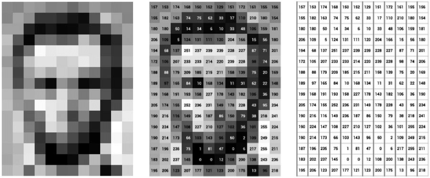
Fig 1: Representation of an Image as Numerical Value or Embedded Image
Image embedding is a vector that represents an image in a certain vector space. They can be represented as either sparse or dense vectors. The former only stores non-zero elements, making it memory efficient, but it may lose out on information. Conversely, the latter provides information down to the minute details of an image and provides better assistance with complex tasks.
Earlier image models relied on manual encoding, which was tedious. However, modern encoders use complex deep-learning algorithms to capture complex image data and patterns. The neural networks can understand minute details and create subtle connections for improved efficiency and accuracy.
Traditional Image Embedding Methods
Traditional image processing techniques were limited and best suited for small and specific datasets. Early techniques used Color Histograms and the concept of a Bag of Visual Words.
Color Histogram maps out frequencies of each image pixel representing a certain color. These are then used to identify or retrieve images, as similar images would have similar Color Histogram compositions. Even though this technique is impressive, we cannot rule out the possibility that two images have similar color compositions, resulting in ambiguity. Moreover, we cannot use this technique to classify based on spatial features.

The concept of a Bag of Visual Words is a dictionary for the most prominent features among the images, which are then clustered into different categories defining a certain class. This dictionary acts as a bag of visual words, where the image is compared with these words. The image is then embedded based on the most frequent features present in the image among the bag of visual words. The drawback of this technique is that we can potentially have a high-frequency count of irrelevant features from a bag of visual words, leading to false information and misinterpretation.

Even though these techniques were not very successful, they were still the leading steps in the evolution of image embeddings.
Breakthroughs with Deep Learning
Deep learning models such as CNN (Convolution Neural Networks) can be trained on large datasets such as ImageNet. This approach results in efficient models that generate effective embeddings with the highest accuracy. ImageNet is a dataset consisting of millions of annotated images for model training. These images are categorized into multiple classes and subclasses and annotated using the WordNet dataset.
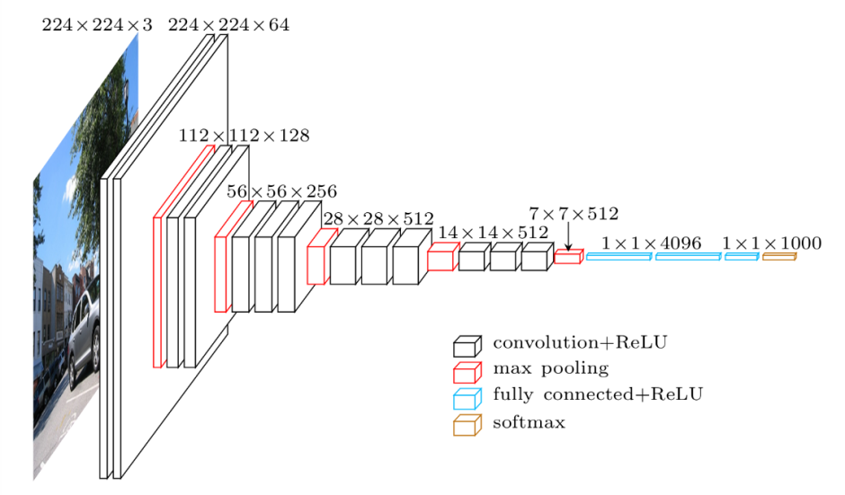
Fig 4: The architecture of VGG-16, a CNN model introduced in 2014.
CNN comprises two blocks: a convolution block and a classification block. The convolution block is responsible for scaling down the complex image into a lower-dimension dense vector, which stores all the information of an image. This information includes spatial features, color composition, texture details, etc. Following the convolution block, the generated output is a dense vector encapsulating the image's essence. This embedded representation then proceeds to the classification block, where the image is attributed with a label corresponding to the desired class. The classification process involves comparing the outcome of the classification block with the actual class label.
The Rise of Transformers in Image Processing
ViT (Vision Transformers) are machine learning (ML) models that use self-attention and positional embedding techniques to classify and process input data. By dividing images into patches and feeding them through internal layers, ViT computes vectors from these patches, comparing them with other vectors to generate alignment scores. Additionally, two extra embeddings are included within layers: a class embedding for classification and a positional embedding to maintain patch sequence integrity.
ViT's patch-based design allows for parallel input, facilitating rapid model training and pre-training on large datasets. These pre-trained models can then be fine-tuned to adapt to specific use cases.
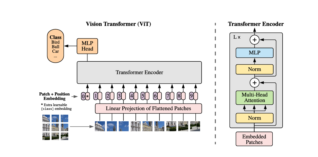
Fig5: Overview of the ViT model
ViT v/s CNN
CNN processes images by analyzing every pixel, while ViT processes images by splitting them into smaller patches. The vector generated by CNN is dense and holds information about every aspect of the image, whereas, in ViT, the vector of different patches is used to compute alignment scores. ViT provides a fast computation advantage as it processes the whole image sequentially, while CNN has to work on every pixel individually.
Multi-Modal Approaches with CLIP
CLIP (Contrastive Language-Image Pretraining) is an advanced machine-learning model that identifies images using textual data and visual inputs. CLIP has two different transformers, one for encoding text embedding vectors and the other for encoding image embedding vectors. These vectors lie in similar vector space and correspond to similar visual and text data.
CLIP is trained on text-image pairs conveying similar meanings. For example, consider an image of a red apple, where the text describing it would be “A sweet red apple.” This pair will be passed to CLIP, where a similar vector will be generated via text and image transformers. This concept has helped improve image search.

CLIP enables zero-shot object classification and detection, requiring no prior training to detect and classify objects. This has opened up many applications:
CLIP can locate and classify objects within images based solely on textual descriptions, even for object classes it hasn't been explicitly trained on.
The zero-shot capability of CLIP helps retrieve images on a text query, making it applicable to image search systems.
Advanced Embedding Techniques
One interesting breakthrough in the CV space is diffusion models. These models generate images from a provided input text or reference image.

Diffusion models are trained by adding noise to the input data on each layer. Once the last layer is reached, they aim to reconstruct the actual or similar data as the input by denoising the generated output.
The Integration of Embedding Models with Vector Databases
Embedding models generate numerical vector representations of input data. Such vectors are stored in specialized stores known as vector databases. We can retrieve images based on our query using image embeddings stored in vector databases like Milvus and Zilliz Cloud (fully managed Milvus vector database).
The difference between a precise search by traditional databases and a vector search by vector databases is that a precise search retrieves results by exactly mapping to the given query. However, a vector search retrieves results similar to the given query. This similarity search is achieved by using the Approximately Nearest Neighbors (ANN) algorithm. Vector databases use this algorithm to map and retrieve vectors with similar spaces. For this reason, we can have multiple results for a specific query, all of which relate to the generated query.
Vector databases help store and index unstructured and semi-structured data. The specialized algorithms applied to the high-dimensional vectors aid in retrieving information related to a generated query almost instantly.
Building a Robust Image Search System
In this section, we will build an image search system (image-to-image) from scratch using Milvus and Timm. Milvus is a top open-source vector database for AI, supporting nearest neighbor search for millions of entries. At the same time, Timm is a deep-learning library containing a collection of models that will help generate image embeddings.
Setup
The following are the installations required to create an image search system:
!pip install pymilvus --upgrade
!pip install timm
!pip install gdown
Before this, make sure the required dependencies are installed.
Torch
Numpy
sklearn
pillow
Imports
Here are the imports required to get started with the code:
import torch
import gdown
import os
import timm
from sklearn.preprocessing import normalize
from timm.data import resolve_data_config
from timm.data.transforms_factory import create_transform
from pymilvus import MilvusClient
from PIL import Image
Dataset
In this article, we’ll use the Caltech-101 dataset, which includes images of objects from 101 categories. Each image is labeled with a single object. Each category has approximately 40 to 800 images, totaling around 9,000 images. Image sizes vary, typically with edge lengths of 200-300 pixels.
The dataset has a directory structure like this:
+---Caltech-101
|   \---test
|        \---ant
|             \---0.jpg
|             \---1.jpg
|             \---....jpg
|   \---train
|        \---aeroplane
|             \---0.jpg
|             \---1.jpg
|             \---....jpg
The dataset required some preprocessing before it could be downloaded from this drive. This includes the dataset and a CSV file that will be later used for image retrieval. We will download and unzip in the following way:
url = '<drive_url>'
output = 'Caltech-101.zip'
gdown.download(url, output, quiet=False)
After downloading, we can unzip it as shown below:
!unzip -q -o /Caltech-101.zip
We can visualize it with Pandas as follows:
df = pd.read_csv('Caltech-101/image_search.csv')
df.head()
Here’s how it looks:
| ID | Path | Label |
| 0 | ./train/ant/image_0033.jpg | ant |
| 1 | ./train/ant/image_0037.jpg | ant |
| 2 | ./train/ant/image_0013.jpg | ant |
| … | … | … |
We are done with our dataset; now, let’s create our collection in Milvus.
Milvus Collection
Like traditional database engines, Milvus allows you to create databases and assign privileges to specific users to manage them.
The MilvusClient is an easier-to-use wrapper for Pymilvus. It is designed to simplify the process and hide much of the complexity found in the original SDK. The create_collection API from the client creates the collection with other parameters. Here’s the implementation.
client = MilvusClient(uri="example.db")

client.create_collection(
    collection_name="image_embeddings",
    vector_field_name="vector",
    dimension=512,
    auto_id=True,
    enable_dynamic_field=True,
    metric_type="COSINE",
)
The code above specifies the collection and vector field names. The collection ID will be automatically generated. It will serve as a primary key dimension 512 for the embedding field.
Embeddings using Timm
Our text-image search system extracts embeddings from images and text using a deep neural network. It then compares these embeddings with those stored in Milvus.
We utilize Timm (short for "PyTorch Image Models"), a popular library in the PyTorch ecosystem to achieve this. It offers a collection of state-of-the-art pre-trained image classification models and utilities for training and evaluation.
This section will leverage Timm’s Resnet-34 to extract embeddings from the images. In the code below, we will define our FeatureExtractor class, which will load the model and necessary configurations and then pass the image to the model after preprocessing it.
class FeatureExtractor:
    def __init__(self, modelname):
        # Load the pre-trained model
        self.model = timm.create_model(
            modelname, pretrained=True, num_classes=0, global_pool="avg"
        )

        self.model.eval()

        self.input_size = self.model.default_cfg["input_size"]

        config = resolve_data_config({}, model=modelname)

        self.preprocess = create_transform(**config)

    def __call__(self, imagepath):
        input_image = Image.open(imagepath).convert("RGB")

        input_image = self.preprocess(input_image)

        input_tensor = input_image.unsqueeze(0)

        with torch.no_grad():

            output = self.model(input_tensor)

        feature_vector = output.squeeze().numpy()

        return normalize(feature_vector.reshape(1, -1), norm="l2").flatten()
Insertion of Image Embeddings in Milvus
In this section, we will utilize the previously defined FeatureExtractor to perform inference on the model, processing the images within the specified directory.
extractor = FeatureExtractor("resnet34")
root = "./Caltech-101/train"

for dirpath, foldername, filenames in os.walk(root):
    for filename in filenames:
        if filename.endswith(".jpg"):
            filepath = dirpath + "/" + filename
            image_embedding = extractor(filepath)
            client.insert(
                    "image_embeddings",
                    {"vector": image_embedding, "filename": filepath},
                )
Alright, we are done with inserting the embeddings in Milvus. Let’s check it on the test dataset.
Query Image on Milvus
In this section, we will query Milvus using the search API. As the search metric, we will specify the collection, query image, and COSINE distance.
query_image = "./test/laptop/image_0001.jpg"

results = client.search(
    "image_embeddings",
    data=[extractor(query_image)],
    output_fields=["filename"],
    search_params={"metric_type": "COSINE"},
)
Testing and Optimizing your Image Search System:
Testing is a hard process for image search in the industry. Here are some steps that can be employed to test the system:
Diverse dataset selection: Choose a diverse dataset representing the images your system is expected to handle. Include images from different categories, styles, resolutions, and lighting conditions.
Ground truth annotation: To evaluate the retrieval system's accuracy, annotate the dataset with ground truth labels or annotations. This can include relevant metadata such as categories, tags, or descriptions.
Benchmarking: Compare your system's performance against existing benchmarks or state-of-the-art methods to assess its relative effectiveness and identify areas for improvement.
Real-world scenarios: Test the system under real-world scenarios that mimic actual usage conditions. Consider factors such as varying input query types, complexity, and user behavior patterns.
User feedback: Incorporate user feedback into the evaluation process to iteratively improve the system.
Once the system is tested, it might also be visible that optimizations are required. Here are some of the tips to optimize the Image search system:
Choosing an effective data type: To optimize storage efficiency when storing embeddings, it's crucial to leverage the full capacity of the data type employed. In many instances, utilizing data types like
FLOAT16_VECTOR, such as in Milvus, proves to store embeddings with half-precision, thereby achieving optimal memory and bandwidth utilization.The trade-off between better and average models: Many people jump to models far superior to others, but such models are hardly scalable. Pick embedding models that can do the job. For example, look at the two variants of CLIP
ViT-B/16andViT-B/32and choose the smaller size to generate embeddings quickly (in this case,ViT-B/16).Always use a GPU: GPUs are efficient in parallel processing and can significantly improve system efficiency. This enables the distribution of training processes and can significantly speed embedding operations.
Create indexes: A database index is a type of data structure that quickly accesses records in a database. Here, we will index on the embedding column of type IVF_FLAT, a quantization-based index that uses approximate nearest neighbor search (ANNS) to provide fast searches. Here is how to create an index in Milvus:
index_params = MilvusClient.prepare_index_params()
index_params.add_index(metric_type='COSINE',
Index_type="IVF_FLAT",
params={"nlist":512}
)
client.create_index(collection_name="...",index_params=index_params)
There are many other indexes that you can use depending on your use case. Here is a full list of it on Milvus.
Use Cases and Real-world Applications
Image embeddings help greatly in image search systems, and some of its applications are listed below:
Image embeddings in e-commerce enable the capability to search for a product by providing a similar image, akin to the functionality in Mozat. Mozat's Image Search system allows users to find similar clothing items from their digital closet, suggests outfit combinations, and provides tailored fashion photo recommendations based on browsing history and closet contents.
Image embeddings and vector databases can detect image anomalies during manufacturing. Identifying low similarity scores ensures quality control.
Text-to-image searches offer users a valuable means to obtain precisely what they desire. Airbnb converts text descriptions into relevant rental properties using image embeddings and vector databases.
Conclusion
In the article, we discussed image embeddings and its various techniques. Traditional methods like color histograms and Bag of Visual Words had shortcomings that led to the development of advanced techniques such as CNNs and transformers. These new approaches served well in the image search field and have built the foundation of most modern embedding models.
Later, diffusion models like DALL-E and Imagen joined the race. Such models generate realistic images from scratch using text descriptions.
The field of AI is moving quickly and is the same for all kinds of data, whether text, image, or video. Read the resources below and experiment with different embedding techniques to stay ahead.
 Haziqa SajidFreelance Technical Writer
Digital Storytelling for Data, AI, B2B & SaaS