Learn
Embedding 101

Unlocking the Power of Vector Quantization: Techniques for Efficient Data Compression and Retrieval

Nov 22, 202415 min read

Vector Quantization (VQ) is a data compression technique representing a large set of similar data points with a smaller set of representative vectors, known as centroids.

By Benito Martin

Read the entire series

Introduction

In today’s data-driven world, managing massive datasets, particularly high-dimensional data like vector embeddings used in various AI applications, has presented significant storage, computation, transmission, and retrieval challenges. Data compression has become a critical strategy for reducing information size without sacrificing utility, enabling faster processing and cost-effective storage.

One compression technique that has proven invaluable in this area is Vector Quantization (VQ). At its core, vector quantization clusters similar data points in a high-dimensional space and represents each cluster with a centroid vector. This approach significantly reduces data size while preserving essential features, making it ideal for applications like image compression, audio processing, and machine learning. In this blog, we’ll explore the principles and techniques of vector quantization and how it enables smarter data compression and efficient retrieval in modern AI-driven systems.

Data Types

To understand vector quantization, it’s important to first grasp the basics of different data types, particularly how quantization reduces data size.

Floating-point numbers represent real numbers in computing, allowing for the expression of an extensive range of values with varying precision. These numbers are stored using bits, which are divided into three main components: the sign (indicating positive or negative), the exponent (scaling the number), and the mantissa or significand (representing the actual digits). By approximating these values during quantization, VQ effectively compresses data while retaining its essential features.

Sign: The sign bit represents whether the number is positive or negative. It’s a single bit, where 0 denotes positive and 1 denotes negative.
Exponent: The exponent determines the scale of the number, allowing for a wide range of values by shifting the decimal point. This flexibility enables the representation of both very large and very small numbers.
Mantissa (significand): The mantissa is the precision part of the floating-point number. It contains the significant digits (the fractional part) of the number, representing the actual value.

For example, the Float32 (or FP32) data type (see Figure 1) is represented by 32 bits or 4 bytes (since 1 byte = 8 bits). It’s also known as a single-precision floating point. This format provides a high level of precision, but it can be computationally expensive and requires a significant amount of memory, especially when dealing with large datasets or high-dimensional vectors.

Figure 1 - Standard floating-point representation (FP32).png

Figure 1: Standard floating-point representation (FP32)

This representation allows for a wide range of values. However, as the dimensionality of the data increases (for instance, high-dimensional embeddings stored and searched in the Milvus vector database), the memory and computational costs become significant. Figure 2 illustrates the memory required by comparing FP32 with two other data types commonly used in vectors: FP16 (16 bits) and INT8 (8 bits).

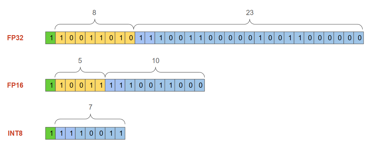Figure 2 - Number formats comparison.png

Figure 2: Number formats comparison

Assuming we have a vector with 512 dimensions, we can calculate the memory required to store it using the following formulas:

equation

Data Type	Bits	Memory for 512-dimensional Vector	Memory for 512-dimensional Vector
FP32	32 bits	2,048 bytes	2 KB
FP16	16 bits	1,024 bytes	1 KB
INT8	8 bits	512 bytes	0.5 KB

Figure 3: Memory requirements for a 512-dimensional vector

However, there is a trade-off between memory efficiency and precision as reducing the bit-width (e.g., from FP32 to INT8) sacrifices some level of precision. On the other hand, as we scale up and store thousands or millions of vectors, maintaining full precision for each vector becomes computationally expensive or even impractical. In such scenarios, a balance between memory usage and precision is required. This is where Vector Quantization (VQ) comes in as a powerful data compression technique to reduce the size of these high-dimensional data points.

Understanding Vector Quantization

Vector Quantization (VQ) is a data compression technique representing a large set of similar data points (input vectors) with a smaller set of representative vectors, known as codewords or centroids. During this process, the input vectors are grouped into clusters (or Voronoi regions), each assigned a codeword that serves as its representative. The collection of all the codewords used to represent the data is called the codebook.

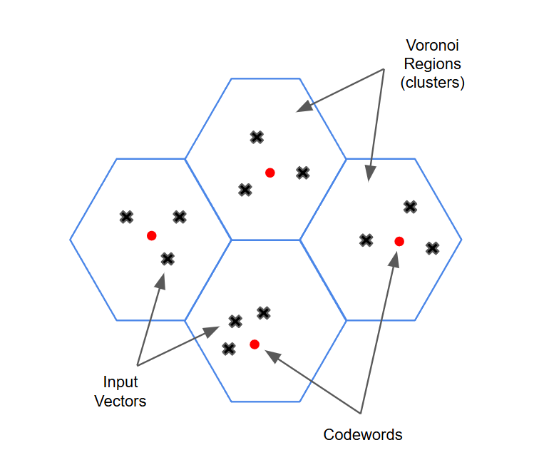Figure 4 - Vector Quantization Diagram

Figure 4: Vector Quantization Diagram

Figure 4 shows a diagram of how vector quantization is being performed. To illustrate this concept in the context of vector databases like Milvus, imagine you have a vast collection of high-dimensional vectors, such as word embeddings from a natural language processing model. When you build the vector database index, rather than using the original vectors, you can use VQ to identify the most representative vectors (centroids) and use only those, which results in significant memory savings. These quantized vectors build the index for faster search and retrieval.

Next, let's simulate a scenario where we create 256 clusters from a set of high-dimensional vectors and then quantize them from 32-bit to 16-bit precision. Each vector is replaced by its index in a codebook of 256 codewords (clusters), and the memory for both the quantized vector indices and the codebook is calculated. This scenario achieves almost 75% memory footprint reduction.

import numpy as np

# Generate some sample high-dimensional vectors
num_vectors = 1000
vector_dim = 1024

# Without quantization
bits32 = 32  # 32-bit float
non_quantized_size = num_vectors * vector_dim * (bits32 / 8) / 1024  # in KB
print(f"Memory required for non-quantized vectors: {non_quantized_size:.2f} KB")

# Quantization details
num_clusters = 256  # Number of clusters in the codebook (codebook size)

# Memory used by quantized vector indices (uint16) and the codebook (4 bytes per centroid dimension)
bits16 = 16  # 16-bit indices
quantized_indices_16 = num_vectors * (bits16 / 8)  # in bytes
codebook_memory_16 = num_clusters * vector_dim * 4  # each codeword is 4 bytes (float32 centroids)

# Total quantized memory in KB
quantized_size_16 = (quantized_indices_16 + codebook_memory_16) / 1024  # in KB
print(f"Memory required for 16-bit quantized vectors: {quantized_size_16:.2f} KB")

# Calculate memory savings for 16-bit quantization
savings_16 = (non_quantized_size - quantized_size_16) / non_quantized_size * 100
print(f"Memory savings with 16-bit quantization: {savings_16:.2f}%")

"""
Output:

Memory required for non-quantized vectors: 4000.00 KB
Memory required for 16-bit quantized vectors: 1025.95 KB
Memory savings with 16-bit quantization: 74.35%
"""

Key Techniques in Vector Quantization

Now that we have a clear idea of Vector Quantization, let’s go deeper into common techniques used within vector databases like Zilliz Cloud and Milvus.

Scalar Quantization

Scalar quantization is the simplest and most straightforward, transforming floating-point numbers into integers. Generally, most embedding models output float32 data types, and vector databases like Zilliz Cloud and Milvus can transform them into int8 integers when performing quantization. The int8 data type uses 8 bits, with a range from -128 to 127, which means that the original floating-point values are mapped to integers within this range.

Data Type	Bits	Range	Range
FP32	32 bits	-2’147’483’648	2’147’483’647
FP16	16 bits	-32’768	32’767
INT8	8 bits	-128	127

Figure 5: Int8 ranges

The transformation is done through normalization based on the minimum and maximum values of the original data. By scaling down to int8, databases like Zilliz Cloud and Milvus can achieve significant memory savings, reducing disk, CPU, and GPU memory consumption by 70–75%.

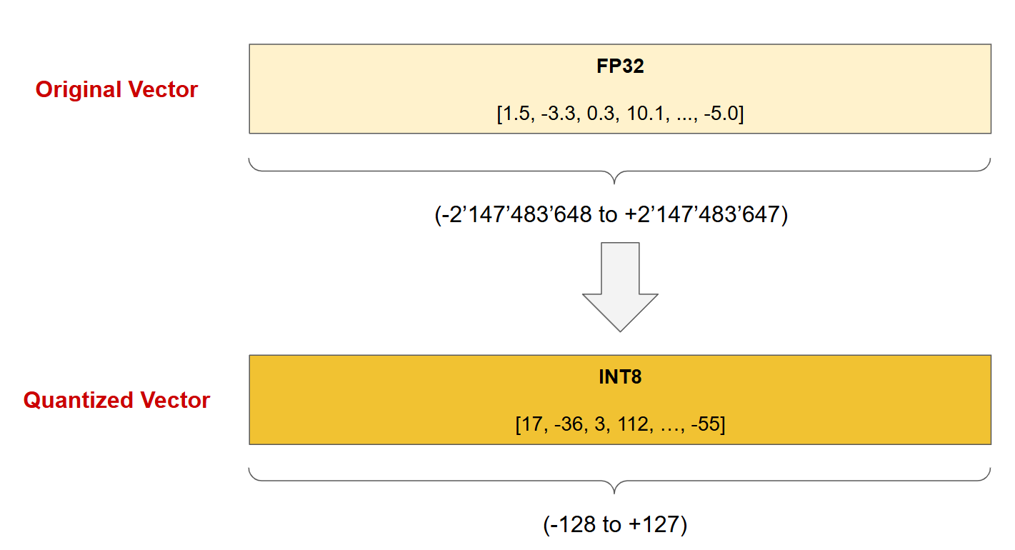Figure 6 - Scalar Quantization.png

Figure 6: Scalar Quantization

This approach trades off some precision but results in reduced storage requirements, for instance, depending on the settings, the scalar quantization index from Milvus IVF_SQ8 can achieve up to 99% recall rate compared to a non-quantized index, making it highly efficient for large-scale systems where speed and storage are prioritized over absolute precision.

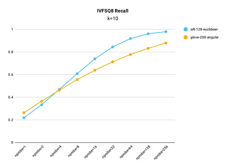Figure 7 - Recall rate test results for IVF_SQ8 index in Milvus.png

Figure 7: Recall rate test results for IVF_SQ8 index in Milvus (Source)

Product Quantization (PQ)

Product Quantization (PQ) is a more advanced compression technique than scalar quantization. Instead of transforming each dimension individually, PQ splits the original high-dimensional vector into a set of smaller, equal-length subvectors. This decomposition allows the algorithm to handle smaller data segments, making compression more manageable and effective, especially in high-dimensional spaces.

Once the vector is divided into subvectors, the K-means clustering algorithm is applied to each subvector group (subspace). Through clustering, a set of centroids (or "codewords") is defined for each subspace, generating its own codebook. Each subvector is then mapped to its closest centroid. This process is repeated across all subvectors, allowing PQ to represent the entire vector as a combination of several centroids from each subspace.

The resulting compressed representation is a sequence of indices referencing the closest centroids in each group, significantly reducing memory usage. For example, in Figure 8, for each original vector with 1024 dimensions of type FP32 (4’096 bytes per vector), if we split the vector into 256 subvectors, and use 8 bits (1 byte) to represent each centroid ID, the quantized vector requires only 256 bytes, which represents a compression rate of 16 (4’096/256).

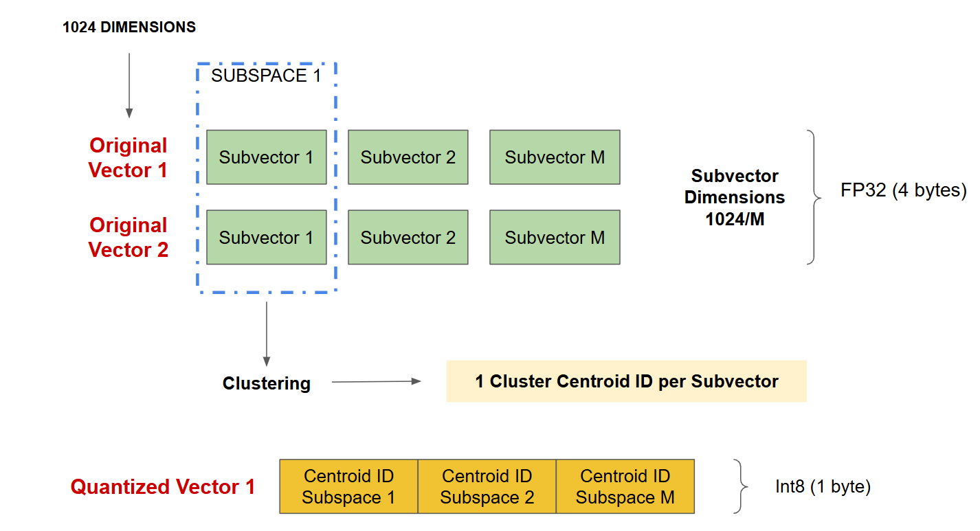Figure 8 - Product Quantization.png

Figure 8: Product Quantization

This technique provides high compression while preserving the structure of the data, making it effective for applications where efficient storage and fast retrieval are essential. However, PQ shows a higher impact on precision than scalar quantization, and the higher the compression, the higher the losses. Milvus currently supports two indexes that perform PQ, IVF_PQ and SCANN (Scalable Nearest Neighbors), the latest applying a combination of PQ with other techniques like anisotropic vector quantization, adapting compression based on data distribution and SIMD (Single Instruction Multiple Data) operations for faster retrieval.

Binary Quantization

Binary quantization is another method that compresses data by converting vector dimensions into a binary representation using only single bits. In this approach, each dimension of the original vector is assigned a binary value: positive values are represented by 1, and negative values are represented by 0. This binary encoding significantly reduces storage requirements since each dimension is represented by a single bit (0 or 1) instead of the original floating-point or integer value.

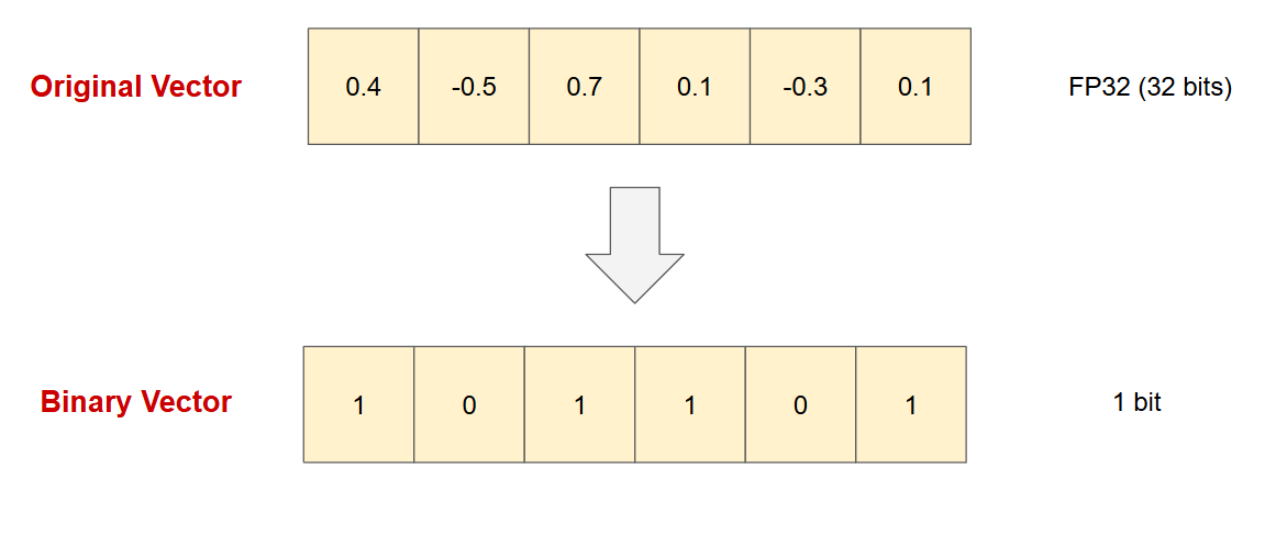Figure 9 - Binary Quantization.png

Figure 9: Binary Quantization

While binary quantization significantly reduces the memory footprint up to 32 times and increases the search speed, it is mostly suitable in high dimensional applications and with specific models pre-tested with binary vectors. Not all models and dimension sizes perform well in terms of accuracy, and the performance shall be tested individually for each model. Additionally, combining binary quantization with rescoring techniques can enhance the final accuracy.

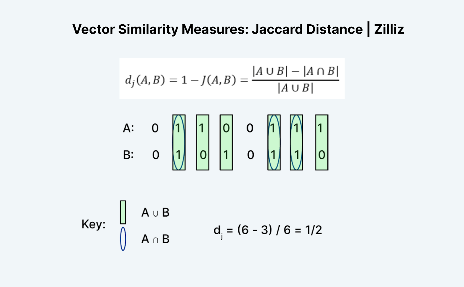Figure 10 - Jaccard Distance.png

Figure 10: Hamming Distance (Source)

In Milvus, binary quantization is supported through two index types:

BIN_FLAT: A binary indexing method that depends on relatively small (million-scale) datasets.
BIN_IVF_FLAT: An inverted file index optimized for High-speed query.

These indices are optimized for binary vectors but unlike high-dimensional vectors that support metrics like cosine similarity, inner product or Euclidean distance, they support two different distance metrics:

Hamming: Measures the number of differing bit positions between two binary vectors, useful for assessing exact bit-level similarity.
Jaccard: Considers the intersection and union of two binary vectors, assessing the proportion of matching bits.

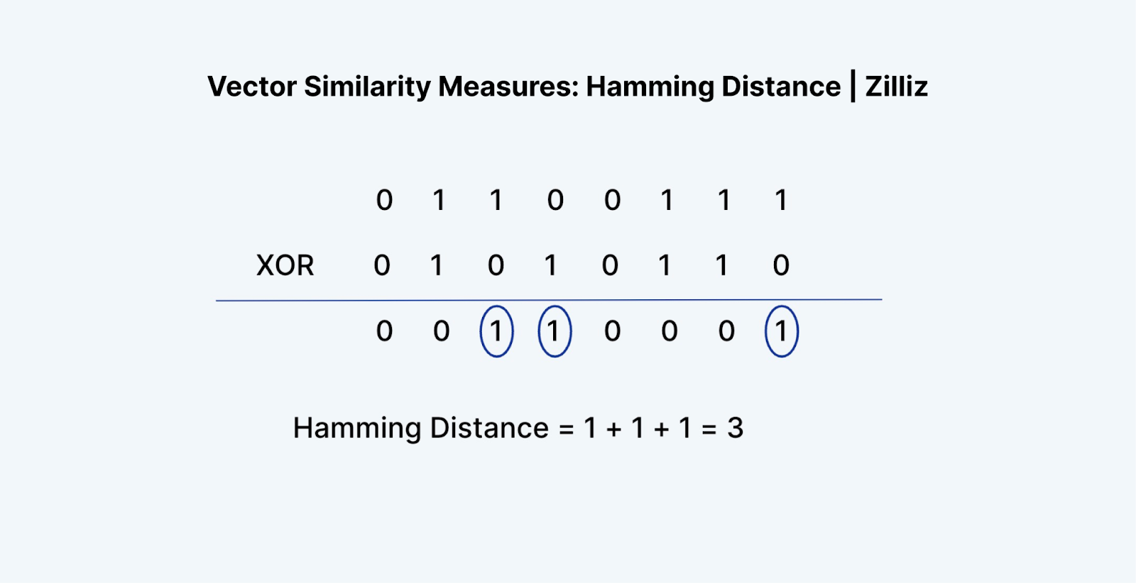Figure 10 - Hamming Distance.png

Figure 10: Jaccard Distance (Source)

Other Techniques in Vector Quantization

The previous sections covered the fundamental techniques of Scalar, Product, and Binary Quantization, which are commonly applied in vector databases like Zilliz Cloud and Milvus. However, the field of vector quantization (VQ) encompasses a broader set of advanced algorithms that are widely used across various applications beyond just vector databases.

In this section, we'll explore several additional VQ techniques, including Lloyd's Algorithm, Linde-Buzo-Gray Algorithm, Residual Quantization, and Tree-Structured Vector Quantization.

Lloyd’s Algorithm (naive K-Means Clustering)

Lloyd’s Algorithm, commonly referred to as naive K-Means clustering, is a fundamental technique in VQ that organizes data points into distinct clusters, each represented by a centroid. The algorithm seeks to reduce the total distance between the data points and their assigned centroids.

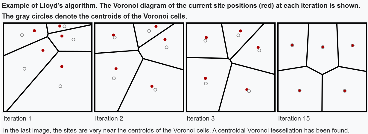Figure 11 - Lloyd’s Algorithm.png

Figure 11: Lloyd’s Algorithm (Source)

Figure 11 illustrates the Voronoi diagram, which visually represents the clusters formed during Lloyd’s Algorithm. Each region corresponds to the area closest to a specific centroid, effectively showing how the algorithm partitions the space such that each point is closer to its assigned centroid than to any other.

The algorithm operates through an iterative process:

Initialization: Begin by randomly selecting initial centroids for a specified number of clusters (k).
Assignment Step: For each data point, assign it to the nearest centroid, determined by a chosen distance metric, such as Euclidean distance.
Update Step: Recalculate each centroid by averaging the data points currently assigned to its cluster.
Repeat: Steps 2 and 3 are repeated until convergence, which occurs when either:

The change in centroid positions falls below a predefined threshold
A maximum number of iterations is reached
Data points maintain stable cluster assignments

Linde-Buzo-Gray (LBG) Algorithm

The Linde-Buzo-Gray (LBG) Algorithm is an extension of Lloyd's Algorithm specifically designed for vector quantization. LBG is particularly effective in scenarios where a high degree of precision is required in data compression, such as speech or image data, and it is widely used in speech and image processing.

The LBG algorithm follows a similar iterative process as Lloyd's but with an important distinction: it uses a binary splitting approach to generate the initial centroids, ensuring a more structured and balanced clustering outcome. The steps are as follows:

Start with a Single Centroid: Calculate the mean of the entire dataset as the first centroid.
Split the Centroids: Split each existing centroid into two by adding and subtracting a small value (perturbation), doubling the number of clusters at each iteration.
Apply Lloyd’s Algorithm: Refine the clusters using Lloyd’s algorithm until convergence.
Repeat: Continue splitting and refining until the desired number of clusters (codebook size) is achieved.

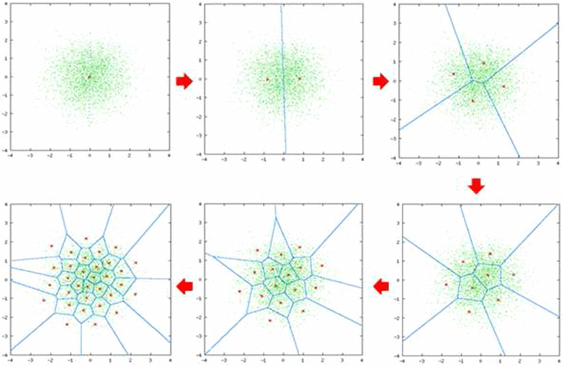Figure 12 - Linde–Buzo–Gray.png

Figure 12: Linde–Buzo–Gray (Source)

Using binary splitting, the LBG algorithm achieves more robust clustering and better data representation with a compact codebook than random initialization methods.

Residual Quantization (RQ)

Residual Quantization (RQ) is a hierarchical VQ method that uses multiple quantization stages to progressively refine each vector's approximation. Particularly effective for high-dimensional data, RQ does not rely on a single centroid to represent each vector but instead represents each vector as a sequence of residuals (errors) from previous approximations.

Here's how it works:

First Quantization: Each vector is first approximated by the closest centroid from an initial codebook.
Calculate Residuals: The difference (residual) between the original vector and its approximation is computed.
Further Quantization: The residuals are quantized with a secondary codebook to capture finer details.
Repeat: This process is repeated across several quantization stages, with each stage capturing residuals from the previous approximation.

The final vector representation is the sum of all quantization stages, allowing for increasingly accurate approximations with each additional stage.

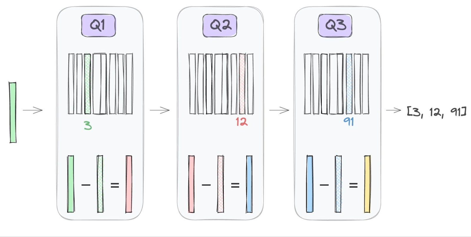Figure 13 - Residual Quantization.png

Figure 13: Residual Quantization (Source)

Tree-Structured Vector Quantization (TSVQ)

Tree-Structured Vector Quantization (TSVQ) organizes vectors in a hierarchical tree structure, where each node represents a different level of quantization granularity. TSVQ allows for efficient, hierarchical searching and data compression by traversing the tree from a root node down to a leaf node that most accurately represents each vector.

The process involves:

Binary Splitting: Similar to LBG, TSVQ starts by splitting a set of vectors into two clusters, which form the root of the tree.
Recursive Splitting: Each cluster is split recursively, generating a tree structure where nodes represent progressively refined quantization levels.
Tree Traversal: When encoding a vector, TSVQ finds the best-fitting cluster by following the branches of the tree from root to leaf. Each leaf node serves as a unique cluster centroid.

Challenges and Considerations

Trade-off Between Compression and Accuracy

One of the primary challenges in VQ is finding the right balance between data size reduction and preserving the quality of information. While higher compression rates can dramatically reduce memory usage, they often come at the cost of accuracy. For instance, lowering the bit width from FP32 to INT8 or applying Product Quantization may introduce quantization errors, causing loss of finer details in high-dimensional data. In applications like image recognition or large language models, this loss of detail could degrade retrieval quality, resulting in less precise outcomes.

Finding the right balance between the degree of compression and the acceptable level of accuracy is crucial. Depending on your needs, the vector quantization parameters may need to be carefully tuned to optimize this tradeoff. For some use cases, a higher compression ratio may be prioritized, even if it means decreased precision. In others, preserving the fidelity of the original data may take precedence over maximizing memory savings. Thus, a careful assessment is needed to determine acceptable information loss in each use case.

Computational Overhead

The process of vector quantization, particularly the initial clustering and centroid calculation steps, can be computationally intensive, especially when dealing with high-dimensional data. However, once the codebook has been established, the search and retrieval process can become more efficient. By representing high-dimensional vectors with a smaller set of centroids, the search space is significantly reduced, leading to faster query processing times. This is a key benefit of VQ, as it enables more efficient search and retrieval of data, even with large-scale high-dimensional datasets.

Therefore, the computational overhead is front-loaded during the initial quantization phase, but the resulting compressed representations can lead to substantial performance improvements during the critical online usage of the system. Careful optimization of VQ and the search process is crucial to ensuring the overall computational efficiency of the vector quantization-based solution.

Application-Specific Tuning

The effectiveness of VQ and the appropriate techniques can vary significantly depending on the specific data types, dimensionality, and intended application. For example, the optimal quantization parameters for compressing text embeddings may differ from those for compressing image feature vectors.

Successful deployment of VQ often requires careful experimentation and tuning to find the right balance of compression, accuracy, and computational efficiency for the target use case. Iterative refinement and ongoing monitoring are crucial to ensuring that the VQ strategy continues to meet the application's needs.

Conclusion

Recap: Key Methods in Vector Quantization

Scalar Quantization Converts floating-point numbers (e.g., FP32) to simpler formats like INT8. This shrinks data by mapping values to a smaller range, saving storage but with slight loss in precision.
Product Quantization (PQ) Splits high-dimensional vectors into smaller chunks, compressing each separately using centroids. This is great for large datasets but may reduce accuracy slightly.
Binary Quantization Turns data into binary values (0s and 1s). While it's ultra-efficient, it works best for specific models and applications.
Residual Quantization Refines data step-by-step by focusing on what's left over after each compression stage. It’s ideal for handling high-dimensional vectors with minimal loss.
Tree-Structured Vector Quantization (TSVQ) Organizes vectors in a tree for efficient searching. Each level represents more refined clusters, making retrieval faster.

Challenges to Consider

Compression vs. Accuracy: Compressing too much can reduce precision, especially in tasks like image recognition. Striking the right balance is key.
Processing Costs: Initial clustering can be computationally heavy, but it pays off with faster searches later.

Bringing It All Together: VQ’s Role in Modern AI

Vector Quantization is a powerful tool in data compression, especially in the context of high-dimensional vector data. By grouping similar data points and representing them with representative centroids, VQ enables significant reductions in storage and computational costs while retaining essential data patterns. As we’ve explored, various quantization techniques—such as Scalar, Product, and Binary—offer distinct advantages and trade-offs depending on the application requirements for speed, memory efficiency, and precision. Other methods, like the Linde-Buzo-Gray Algorithm and Tree-Structured Vector Quantization, further demonstrate the versatility of VQ in handling large, complex datasets.

These quantization methods are critical for scaling data-intensive tasks in modern applications, particularly those powered by various AI technologies such as large language models (LLMs) and vector databases like Zilliz Cloud and Milvus. While there is always a balance to strike between compression and accuracy, the continued development of VQ methods ensures that we can optimize storage and processing power without compromising too much on precision. As data volumes continue to grow, VQ will remain a vital area of innovation, enabling faster, more efficient storage and retrieval in the era of big data.

Benito Martin
Freelance Technical Writer

Start Free, Scale Easily

Try the fully-managed vector database built for your GenAI applications.

Try Zilliz Cloud for Free