Learn
Vector Database 101: Everything You Need to Know

DiskANN and the Vamana Algorithm

Oct 29, 20236 min read

Dive into DiskANN, a graph-based vector index, and Vamana, the core data structure behind DiskANN.

Read the entire series

Introduction to DiskANN and the Vamana Algorithm

Hey there - welcome back to Milvus tutorials. In the previous tutorial, we did a deep dive into Approximate Nearest Neighbors Oh Yeah, or Annoy for short. Annoy is a tree-based indexing algorithm that uses random projections to iteratively split the hyperspace of vectors, with the final split resulting in a binary tree. Annoy uses two tricks to improve accuracy/recall - 1) traversing down both halves of a split if the query point lies close to the dividing hyperplane, and 2) creating a forest of binary trees. Although Annoy isn't commonly used as an indexing algorithm in production environments today (HNSW and IVF_PQ are far more popular), Annoy still sets a strong baseline for tree-based vector indexes.

At its core, Annoy is still an in-memory index. We've only looked at in-memory indexes - vector indexes that reside entirely in RAM. On commodity machines, in-memory indexes are excellent for smaller datasets (up to around 10 million 1024-dimensional vectors). Still, once we move past 100M vectors, in-memory indexes can be prohibitively expensive. For example, 100M vectors alone will require approximately 400GB of RAM.

Here's where an on-disk index - a vector index that utilizes both RAM and hard disk - would be helpful. In this tutorial, we'll dive into DiskANN, a graph-based vector index that enables large-scale storage, indexing, and search of vectors by persisting the bulk of the index on NVMe hard disks. We'll first cover Vamana, the core data structure behind DiskANN, before discussing how the on-disk portion of DiskANN utilizes a Vamana graph to perform queries efficiently. Like previous tutorials, we'll also develop our implementation of the Vamana algorithm in Python.

The Vamana algorithm

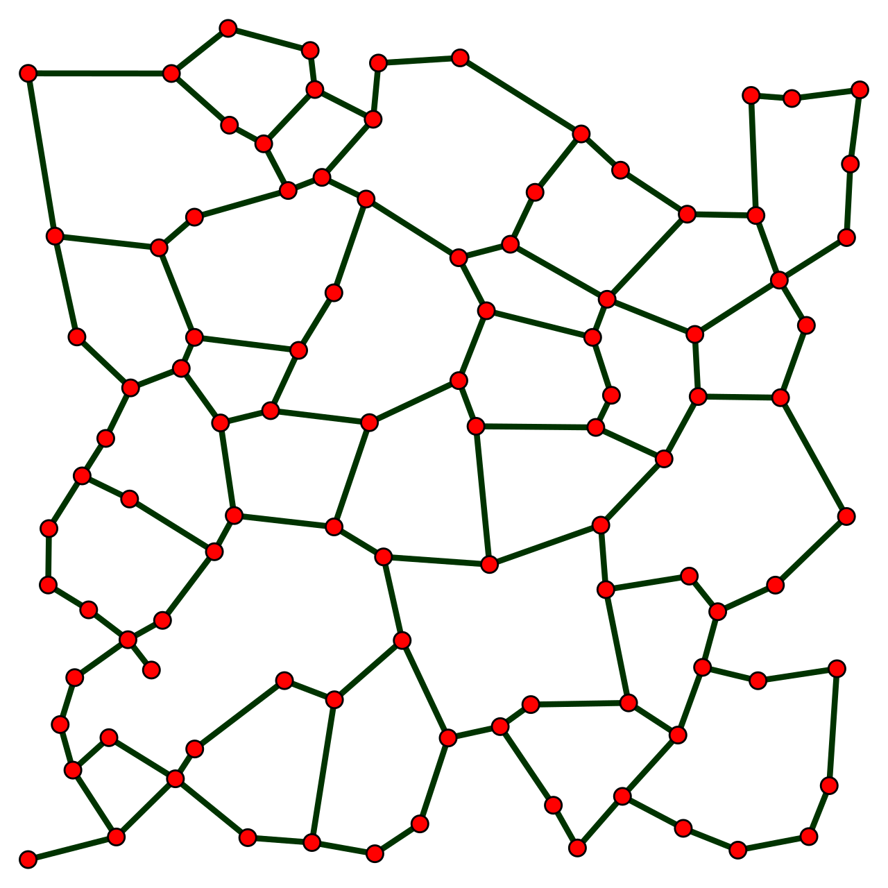
Vamana's key concept is the relative neighborhood graph (RNG). Formally, edges in an RNG for a single point are constructed iteratively so long as a new edge is not closer to any existing neighbor. If this is difficult to wrap your head around, no worries - the key concept is that RNGs are constructed so that only a subset of the most relevant nearest edges are added for any single point in the graph. As with HNSW, nearby vectors are determined by the distance metric that's being used in the vector database, e.g., cosine or L2.

There are two main problems with RNGs that make them still too inefficient for vector search. The first is that constructing an RNG is prohibitively expensive: $O(n^2)$ for a dataset with size $n$ . The second is that setting the diameter of an RNG is difficult. High-diameter RNGs are too dense, while RNGs with low diameters make graph traversal (querying the index) lengthy and inefficient. Despite this, RNGs remain a good starting point and form the basis for the Vamana algorithm.

The relative neighborhood graph of 100 random points in a unit square

Image source: Wikepedia-Relative neighborhood graph. Note how any point is only connected to a subset of its closest neighbors.

In broad terms, the Vamana algorithm solves both of these problems by making use of two clever heuristics: the greedy search procedure and the robust prune procedure. Let's walk through both of these, along with an implementation, to see how these work together to create an optimized graph for vector search.

As the name implies, the greedy search algorithm iteratively searches for the closest neighbors to a specified point (vector) in the graph p. Loosely speaking, we maintain two sets: a set of nearest neighbors nns and a set of visited nodes visit.

def _greedy_search(graph, start, query, nq: int, L: int):

    best = (np.linalg.norm(graph[start][0] - query), entry)

    nns = [start]
    visit = set()  # set of visited nodes
    nns = heapify(nns)

    # find top-k nearest neighbors
    while nns - visit:
        nn = nns[0]
        for idx in nn[1]:
            d = np.linalg.norm(graph[idx][0] - query)
            heappush(nns, (d, nn))
            visit.add((d, nn))

        # retain up to search list size elements
        while len(nns) > L:
            heappop(nns)

    return (nns[:nq], visit)

nns is initialized with the starting node, and at each iteration, we take up to L steps in the direction closest to our query point. This continues until all nodes in nns have been visited.

Robust prune, on the other hand, is a bit more involved. This heuristic is designed to ensure that the distance between consecutive searched nodes in the greedy search procedure decreases exponentially. Formally, robust prune, when called on a single node, will ensure that the outbound edges are modified such that there are at most R edges, with a new edge pointing to a node at least a times distant from any existing neighbor.

def _robust_prune(graph, node: Tuple[np.ndarray, Set[int]], candid: Set[int], R: int):
    
    candid.update(node[1])
    node[1].clear()

    while candid:
        (min_d, nn) = (float("inf"), None)

        # find the closest element/vector to input node
        for k in candid:
            p = graph[k]
            d = np.linalg.norm(node[0] - p[0])
            if d < min_d:
                (min_d, nn) = (d, p)
        node[1].add(nn)

        # set at most R out-neighbors for the selected node
        if len(node[1]) == R:
            break

        # future iterations must obey distance threshold
        for p in candid:
            if a * min_d <= np.linalg.norm(node[0] - p[0]):
                candid.remove(p)

With these two heuristics, we can now focus on the full Vamana algorithm. A Vamana graph is first initialized so each node has R random outbound edges. The algorithm then iteratively calls _greedy_search and _robust_prune for all nodes within the graph.

As we've done for all of our previous tutorials on vector indexes, let's now put it all together into a single script:

class VamanaIndex(_BaseIndex):
    """Vamana graph algorithm implementation. Every element in each graph is a
    2-tuple containing the vector and a list of unidirectional connections
    within the graph.
    """

    def __init__(self, L: int = 10, a: float = 1.5, R: int = 10):
        super().__init__()
        self._L = L
        self._a = a
        self._R = R
        self._start = None  # index of starting vector
        self._index = []


    def create(self, dataset):

        self._R = min(self._R, len(dataset))

        # intialize graph with dataset
        # set starting location as medoid vector
        dist = float("inf")
        medoid = np.median(dataset, axis=0)
        for (n, vec) in enumerate(dataset):
            d = np.linalg.norm(medoid - vec)
            if d < dist:
                dist = d
                self._start = n
            self._index.append((vec, set()))

        # randomize out-connections for each node
        for (n, node) in enumerate(self._index):
            idxs = np.random.choice(len(self._index) - 1, replace=False, size=(self._R,))
            idxs[idxs >= n] += 1  # ensure no node points to itself
            node[1].update(idxs)

        # random permutation + sequential graph update
        for (n, node) in enumerate(self._index):
            (_, V) = self.search(node, nq=1)
            self._robust_prune(node, V)
            for inb in node[1]:
                nbr = self._index[inb]
                if len(nbrs[1]) > self._R:
                    self._robust_prune(nbr, nbr[1].union(n))
                else:
                    nbr[1].add(n)


    def insert(self, vector):
        raise NotImplementedError("Vamana indexes are static")


    def search(query, nq: int = 10):
        """Greedy search.
        """

        best = (np.linalg.norm(self._index[self._start][0] - query), entry)

        nns = [start]
        visit = set()  # set of visited nodes
        nns = heapify(nns)

        # find top-k nearest neighbors
        while nns - visit:
            nn = nns[0]
            for idx in nn[1]:
                d = np.linalg.norm(self._index[idx][0] - query)
                heappush(nns, (d, nn))
                visit.add((d, nn))

            # retain up to search list size elements
            while len(nns) > self._L:
                heappop(nns)

        return (nns[:nq], visit)


    def _robust_prune(node: Tuple[np.ndarray, Set[int]], candid: Set[int]):
        
        candid.update(node[1])
        node[1].clear()

        while candid:
            (min_d, nn) = (float("inf"), None)

            # find the closest element/vector to input node
            for k in candid:
                p = self._index[k]
                d = np.linalg.norm(node[0] - p[0])
                if d < min_d:
                    (min_d, nn) = (d, p)
            node[1].add(nn)

            # set at most R out-neighbors for the selected node
            if len(node[1]) == R:
                break

            # future iterations must obey distance threshold
            for p in candid:
                if a * min_d <= np.linalg.norm(node[0] - p[0]):
                    candid.remove(p)

That's it for Vamana!

Wrapping up

In this tutorial, we did a deep dive into DiskANN, a graph-based indexing strategy that is our first foray into on-disk indexes. Like HNSW, DiskANN avoids the problem of figuring out how and where to partition a high-dimensional input space and instead relies on building a directed graph to the relationship between nearby vectors. As the volume of unstructured data continues to grow in the upcoming decade, the need for on-disk indexes will likely rise, as will research around this area.

All code for this tutorial is freely available at https://github.com/fzliu/vector-search.

Take another look at the Vector Database 101 courses

Frank Liu
Frank Liu is the Director of Operations & ML Architect at Zilliz, where he serves as a maintainer for the Towhee open-source project. Prior to Zilliz, Frank co-founded Orion Innovations, an ML-powered indoor positioning startup based in Shanghai and worked as an ML engineer at Yahoo in San Francisco. In his free time, Frank enjoys playing chess, swimming, and powerlifting. Frank holds MS and BS degrees in Electrical Engineering from Stanford University.

Next: Safeguard Data Integrity: Backup and Recovery in Vector Databases

Content

Start Free, Scale Easily

Try the fully-managed vector database built for your GenAI applications.

Try Zilliz Cloud for Free