


Approximate Nearest Neighbors Oh Yeah (Annoy)
Discover the capabilities of Annoy, an innovative algorithm revolutionizing approximate nearest neighbor searches for enhanced efficiency and precision.
Read the entire series
- Introduction to Unstructured Data
- What is a Vector Database and how does it work: Implementation, Optimization & Scaling for Production Applications
- Understanding Vector Databases: Compare Vector Databases, Vector Search Libraries, and Vector Search Plugins
- Introduction to Milvus Vector Database
- Milvus Quickstart: Install Milvus Vector Database in 5 Minutes
- Introduction to Vector Similarity Search
- Everything You Need to Know about Vector Index Basics
- Scalar Quantization and Product Quantization
- Hierarchical Navigable Small Worlds (HNSW)
- Approximate Nearest Neighbors Oh Yeah (Annoy)
- Choosing the Right Vector Index for Your Project
- DiskANN and the Vamana Algorithm
- Safeguard Data Integrity: Backup and Recovery in Vector Databases
- Dense Vectors in AI: Maximizing Data Potential in Machine Learning
- Integrating Vector Databases with Cloud Computing: A Strategic Solution to Modern Data Challenges
- A Beginner's Guide to Implementing Vector Databases
- Maintaining Data Integrity in Vector Databases
- From Rows and Columns to Vectors: The Evolutionary Journey of Database Technologies
- Decoding Softmax Activation Function
- Harnessing Product Quantization for Memory Efficiency in Vector Databases
- How to Spot Search Performance Bottleneck in Vector Databases
- Ensuring High Availability of Vector Databases
- Mastering Locality Sensitive Hashing: A Comprehensive Tutorial and Use Cases
- Vector Library vs Vector Database: Which One is Right for You?
- Maximizing GPT 4.x's Potential Through Fine-Tuning Techniques
- Deploying Vector Databases in Multi-Cloud Environments
- An Introduction to Vector Embeddings: What They Are and How to Use Them
Introduction
Welcome back to Vector Database 101.
In the previous tutorial, we deep-dived into Hierarchical Navigable Small Worlds (HNSW). HNSW is a graph-based indexing algorithm that today is one of the most popular indexing strategies used in vector databases.
In this tutorial, we'll switch gears and talk about tree-based vector indexes. Specifically, we'll talk about Approximate Nearest Neighbors Oh Yeah (Annoy), an algorithm that uses a forest of trees to conduct the nearest neighbor search. For those familiar with random forests or gradient-boosted decision trees, Annoy can seem like a natural extension of these algorithms, only for the nearest neighbor search rather than machine learning. As with our HNSW tutorial, we'll first walk through how Annoy works from a high level before developing our own simple Python implementation.
Annoy basics
While HNSW is built upon the connected graph and skip list, Annoy uses binary search trees as the core data structure. The key idea behind Annoy (and other tree-based indexes) is to repeatedly partition our vector space and search only a subset of the partitions for nearest neighbors. If this sounds like IVF, you're right; the idea is the same, but the execution is slightly different.
 Annoy, visualized
The best way to understand Annoy is to visualize how a single tree is built. However, remember that high-dimensional hyperspaces are very different from 2D/3D Euclidean spaces from an intuitive perspective, so the images below are only for reference.
Let's start with indexing. For Annoy, this is a recursive process where the maximum size of the call stack is the depth of the tree. In the first iteration, two random dataset vectors, a and b, are selected, and the full hyperspace is split along a hyperplane equidistant from both a and b. Then, vectors in the "left" half of the hyperspace get assigned to the left half of the tree, while vectors in the "right" half of the subspace are given to the right half of the tree. Note that this can be done without actually computing the hyperplane itself - for every dataset vector, we need to determine whether a (left) or b (right) is closer.
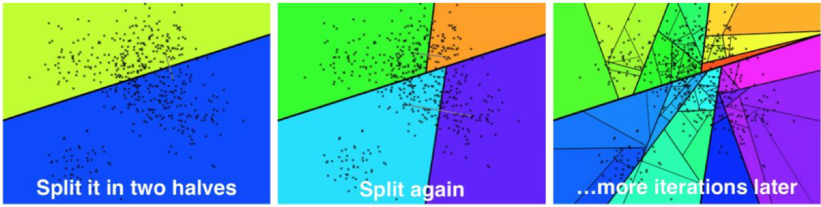
After the first, second, and Nth iteration, respectively. Source.
The second iteration repeats this process for both the left and right subtrees generated by the first iteration, resulting in a tree with a depth of two and four leaf nodes. This process continues for the third, fourth, and subsequent iterations until a leaf node has fewer than a pre-defined number of elements K. In the original Annoy implementation, K is a variable value that the user can set.
With the index fully built, we can now move on to querying. Given some query vector q, we can search by traversing the tree. A hyperplane splits each intermediate node, and we can determine which side of the hyperplane the query vector falls on by computing its distance to the left and right vectors. We repeat this process until we reach a leaf node containing an array of, at most, K vectors. We can then rank and return these vectors to the user.
Implementing Annoy
Now we know how Annoy works, and let's start with the implementation. As usual, we'll first create a dataset of (128 dimensional) vectors:
>>> import numpy as np
>>> dataset = np.random.normal(size=(1000, 128))
Let's first define a Node class containing left and right subtrees:
class Node(object):
    """Initialize with a set of vectors, then call `split()`.
    """

    def __init__(self, ref: np.ndarray, vecs: List[np.ndarray]):
        self._ref = ref
        self._vecs = vecs
        self._left = None
        self._right = None

    @property
    def ref(self) -> Optional[np.ndarray]:
        """Reference point in n-d hyperspace. Evaluates to `False` if root node.
        """
        return self._ref

    @property
    def vecs(self) -> List[np.ndarray]:
        """Vectors for this leaf node. Evaluates to `False` if not a leaf.
        """
        return self._vecs

    @property
    def left(self) -> Optional[object]:
        """Left node.
        """
        return self._left

    @property
    def right(self) -> Optional[object]:
        """Right node.
        """
        return self._right
The vecs variable contains a list of all vectors within the node. If the length of this list is less than some value K, then they will remain as-is; otherwise, these vectors will then get propagated to left and right, with vecs[0] and vecs[1] remaining as the two randomly selected vectors used to split the hyperplane.
Let's now move to indexing. First, Recall that every node in the tree is split by a hyperplane orthogonal to the line connecting two randomly selected dataset vectors. Conveniently, we can determine which side of the hyperplane a query vector lies on by computing distance. As usual, we'll use NumPy's vectorized math for this:
def _is_query_in_left_half(q, node):
   # returns `True` if query vector resides in left half
   dist_l = np.linalg.norm(q - node.vecs[0])
   dist_r = np.linalg.norm(q - node.vecs[1])
   return dist_l < dist_r
Now let's move to building the actual tree.
import random


def split_node(node, K: int, imb: float) -> bool:

    # stopping condition: maximum # of vectors for a leaf node
    if len(node._vecs) <= K:
        return False

    # continue for a maximum of 5 iterations
    for n in range(5):
        left_vecs = []
        right_vecs = []

        # take two random indexes and set as left and right halves
        left_ref = node._vecs.pop(np.random.randint(len(node._vecs)))
        right_ref = node._vecs.pop(np.random.randint(len(node._vecs)))

        # split vectors into halves
        for vec in node._vecs:
            dist_l = np.linalg.norm(vec - left_ref)
            dist_r = np.linalg.norm(vec - right_ref)
            if dist_l < dist_r:
                left_vecs.append(vec)
            else:
                right_vecs.append(vec)

        # check to make sure that the tree is mostly balanced
        r = len(left_vecs) / len(node._vecs)
        if r < imb and r > (1 - imb):
            node._left = Node(left_ref, left_vecs)
            node._right = Node(right_ref, right_vecs)
            return True

        # redo tree build process if imbalance is high
        node._vecs.append(left_ref)
        node._vecs.append(right_ref)

    return False


def _build_tree(node, K: int, imb: float):
    """Recurses on left and right halves to build a tree.
    """
    node.split(K=K, imb=imb)
    if node.left:
        _build_tree(node.left, K=K, imb=imb)
    if node.right:
        _build_tree(node.right, K=K, imb=imb)


def build_forest(vecs: List[np.ndarray], N: int = 32, K: int = 64, imb: float = 0.95) -> List[Node]:
    """Builds a forest of `N` trees.
    """
    forest = []
    for _ in range(N):
        root = Node(None, vecs)
        _build_tree(root, K, imb)
        forest.append(root)
    return forest
This is a denser code block, so let's walk through it step-by-step. First, given an already-initialized Node, we randomly select two vectors and split the dataset into left and right halves. We then use the function we defined earlier to determine which of the two halves the subvectors belong to. Note that we've added an imb parameter to maintain tree balance - if one side of the tree contains more than 95% of all the subvectors, we redo the split process.
With node splitting in place, the build_tree function will recursively call itself on all nodes. Leaf nodes are defined as those which contain fewer than K subvectors.
Great, so we've built a binary tree that lets us significantly reduce the scope of our search. Now let's implement querying as well. Querying is pretty straightforward; we traverse the tree, continuously moving along the left or right branches until we've arrived at the one we're interested in:
def _query_linear(vecs: List[np.ndarray], q: np.ndarray, k: int) -> List[np.ndarray]:
    return sorted(vecs, key=lambda v: np.linalg.norm(q-v))[:k]


def query_tree(root: Node, q: np.ndarray, k: int) -> List[np.ndarray]:
    """Queries a single tree.
    """

    while root.left and root.right:
        dist_l = np.linalg.norm(q - node.left.ref)
        dist_r = np.linalg.norm(q - node.right.ref)
        root = root.left if dist_l < dist_r else root.right

    # brute-force search the nearest neighbors
    return _query_linear(root.vecs, q, k)
This chunk of code will greedily traverse the tree, returning a single nearest neighbor (nq = 1). However, recall that we're often interested in finding multiple nearest neighbors. Additionally, multiple nearest neighbors can live in other leaf nodes as well. So how can we solve these issues?
Run, forest, run
(Yes, I do realize that the main character's name is spelled "Forrest" in the American classic.)
In a previous tutorial on IVF, recall that we often expanded our search beyond the Voronoi cell closest to the query vector. The reason is due to cell edges - if a query vector is close to a cell edge, it's very likely that some of its nearest neighbors may be in a neighboring cell. These "edges" are much more common in high-dimensional spaces, so a large-ish value of nprobe is often used when a high recall is needed.
We face the same problem for tree-based indexes - some of our nearest neighbors may be outside the nearest leaf node/polygon. Annoy solves this by 1) allowing searches on both sides of a split and 2) creating a forest of trees.
Let's first expand on our implementation in the previous section to search both sides of a split:
def _select_nearby(node: Node, q: np.ndarray, thresh: int = 0):
    """Functions identically to _is_query_in_left_half, but can return both.
    """
    if not node.left or not node.right:
        return ()
    dist_l = np.linalg.norm(q - node.left.ref)
    dist_r = np.linalg.norm(q - node.right.ref)
    if np.abs(dist_l - dist_r) < thresh:
        return (node.left, node.right)
    if dist_l < dist_r:
        return (node.left,)
    return (node.right,)


def _query_tree(root: Node, q: np.ndarray, k: int) -> List[np.ndarray]:
    """This replaces the `query_tree` function above.
    """

    pq = [root]
    nns = []
    while pq:
        node = pq.pop(0)
        nearby = _select_nearby(node, q, thresh=0.05)

        # if `_select_nearby` does not return either node, then we are at a leaf
        if nearby:
            pq.extend(nearby)
        else:
            nns.extend(node.vecs)

    # brute-force search the nearest neighbors
    return _query_linear(nns, q, k)


def query_forest(forest: List[Node], q, k: int = 10):
    nns = set()
    for root in forest:
        # merge `nns` with query result
        res = _query_tree(root, q, k)
        nns.update(res)
    return _query_linear(nns, q, k)
Next, we'll add a function to allow us to build the full index as a forest of trees:
def build_forest(vecs: List[np.ndarray], N: int = 32, K: int = 64, imb: float = 0.95) -> List[Node]:
    """Builds a forest of `N` trees.
    """
    forest = []
    for _ in range(N):
        root = Node(None, vecs)
        _build_tree(root, K, imb)
        forest.append(root)
    return forest
With everything implemented, let's now put it all together, as we've done for IVF, SQ, PQ, and HNSW:
from typing import List, Optional
import random

import numpy as np


class Node(object):
    """Initialize with a set of vectors, then call `split()`.
    """

    def __init__(self, ref: np.ndarray, vecs: List[np.ndarray]):
        self._ref = ref
        self._vecs = vecs
        self._left = None
        self._right = None

    @property
    def ref(self) -> Optional[np.ndarray]:
        """Reference point in n-d hyperspace. Evaluates to `False` if root node.
        """
        return self._ref

    @property
    def vecs(self) -> List[np.ndarray]:
        """Vectors for this leaf node. Evaluates to `False` if not a leaf.
        """
        return self._vecs

    @property
    def left(self) -> Optional[object]:
        """Left node.
        """
        return self._left

    @property
    def right(self) -> Optional[object]:
        """Right node.
        """
        return self._right

    def split(self, K: int, imb: float) -> bool:

        # stopping condition: maximum # of vectors for a leaf node
        if len(self._vecs) <= K:
            return False

        # continue for a maximum of 5 iterations
        for n in range(5):
            left_vecs = []
            right_vecs = []

            # take two random indexes and set as left and right halves
            left_ref = self._vecs.pop(np.random.randint(len(self._vecs)))
            right_ref = self._vecs.pop(np.random.randint(len(self._vecs)))

            # split vectors into halves
            for vec in self._vecs:
                dist_l = np.linalg.norm(vec - left_ref)
                dist_r = np.linalg.norm(vec - right_ref)
                if dist_l < dist_r:
                    left_vecs.append(vec)
                else:
                    right_vecs.append(vec)

            # check to make sure that the tree is mostly balanced
            r = len(left_vecs) / len(self._vecs)
            if r < imb and r > (1 - imb):
                self._left = Node(left_ref, left_vecs)
                self._right = Node(right_ref, right_vecs)
                return True

            # redo tree build process if imbalance is high
            self._vecs.append(left_ref)
            self._vecs.append(right_ref)

        return False


def _select_nearby(node: Node, q: np.ndarray, thresh: int = 0):
    """Functions identically to _is_query_in_left_half, but can return both.
    """
    if not node.left or not node.right:
        return ()
    dist_l = np.linalg.norm(q - node.left.ref)
    dist_r = np.linalg.norm(q - node.right.ref)
    if np.abs(dist_l - dist_r) < thresh:
        return (node.left, node.right)
    if dist_l < dist_r:
        return (node.left,)
    return (node.right,)


def _build_tree(node, K: int, imb: float):
    """Recurses on left and right halves to build a tree.
    """
    node.split(K=K, imb=imb)
    if node.left:
        _build_tree(node.left, K=K, imb=imb)
    if node.right:
        _build_tree(node.right, K=K, imb=imb)


def build_forest(vecs: List[np.ndarray], N: int = 32, K: int = 64, imb: float = 0.95) -> List[Node]:
    """Builds a forest of `N` trees.
    """
    forest = []
    for _ in range(N):
        root = Node(None, vecs)
        _build_tree(root, K, imb)
        forest.append(root)
    return forest


def _query_linear(vecs: List[np.ndarray], q: np.ndarray, k: int) -> List[np.ndarray]:
    return sorted(vecs, key=lambda v: np.linalg.norm(q-v))[:k]


def _query_tree(root: Node, q: np.ndarray, k: int) -> List[np.ndarray]:
    """Queries a single tree.
    """

    pq = [root]
    nns = []
    while pq:
        node = pq.pop(0)
        nearby = _select_nearby(node, q, thresh=0.05)

        # if `_select_nearby` does not return either node, then we are at a leaf
        if nearby:
            pq.extend(nearby)
        else:
            nns.extend(node.vecs)

    # brute-force search the nearest neighbors
    return _query_linear(nns, q, k)


def query_forest(forest: List[Node], q, k: int = 10):
    nns = set()
    for root in forest:
        # merge `nns` with query result
        res = _query_tree(root, q, k)
        nns.update(res)
    return _query_linear(nns, q, k)
And that's it for Annoy!
Wrapping up
In this tutorial, we did a deep dive into Annoy, a tree-based indexing strategy with a playful name. There are better languages than Python for implementing vector search data structures due to interpreter overhead. Still, we use as much numpy-based array math. We can do many optimizations to prevent copying memory back and forth, but I'll leave them as an exercise for the reader.
In the following tutorial, we'll continue our deep dive into indexing strategies with a rundown of the Vamana algorithm - also known more commonly as DiskANN - a unique graph-based indexing algorithm that is tailored specifically towards querying directly from solid state hard drives.
All code for this tutorial is freely available on my Github.
Take another look at the Vector Database 101 courses
- Introduction to Unstructured Data
- What is a Vector Database?
- Comparing Vector Databases, Vector Search Libraries, and Vector Search Plugins
- Introduction to Milvus
- Milvus Quickstart
- Introduction to Vector Similarity Search
- Vector Index Basics and the Inverted File Index
- Scalar Quantization and Product Quantization
- Hierarchical Navigable Small Worlds (HNSW)
- Approximate Nearest Neighbors Oh Yeah (ANNOY)
- Choosing the Right Vector Index for Your Project
- DiskANN and the Vamana Algorithm
 Frank Liu
Frank Liu is the Director of Operations & ML Architect at Zilliz, where he serves as a maintainer for the Towhee open-source project. Prior to Zilliz, Frank co-founded Orion Innovations, an ML-powered indoor positioning startup based in Shanghai and worked as an ML engineer at Yahoo in San Francisco. In his free time, Frank enjoys playing chess, swimming, and powerlifting. Frank holds MS and BS degrees in Electrical Engineering from Stanford University.
- Introduction
- Annoy basics
- Implementing Annoy
- Run, forest, run
- Wrapping up
- Take another look at the Vector Database 101 courses
Content
Start Free, Scale Easily
Try the fully-managed vector database built for your GenAI applications.
Try Zilliz Cloud for FreeKeep Reading

Maintaining Data Integrity in Vector Databases
Guaranteeing that data is correct, consistent, and dependable throughout its lifecycle is important in data management, especially in vector databases

Ensuring High Availability of Vector Databases
Ensuring high availability is crucial for the operation of vector databases, especially in applications where downtime translates directly into lost productivity and revenue.

Mastering Locality Sensitive Hashing: A Comprehensive Tutorial and Use Cases
Understand Locality Sensitive Hashing as an effective similarity search technique. Learn practical applications, challenges, and Python implementation of LSH.