Learn
Natural Language Processing (NLP) Advanced Guide

Time Series Embedding in Data Analysis

Apr 09, 202414 min read

Learn about time series data including general concepts and preprocessing methods to transform time series data into an embedding suitable for forecasting tasks.

By Ruben Winastwan

Read the entire series

Time series is a fundamental topic in data science, given its widespread use cases in various business sectors, such as finance, healthcare, supply chain management, manufacturing, etc. In this article, we will discuss everything about time series data. First, we'll cover the general concept of time series data. Then, we'll explore preprocessing methods to transform time series data into an embedding suitable for forecasting tasks. So, let's dive in!

Understanding Time Series Data Points

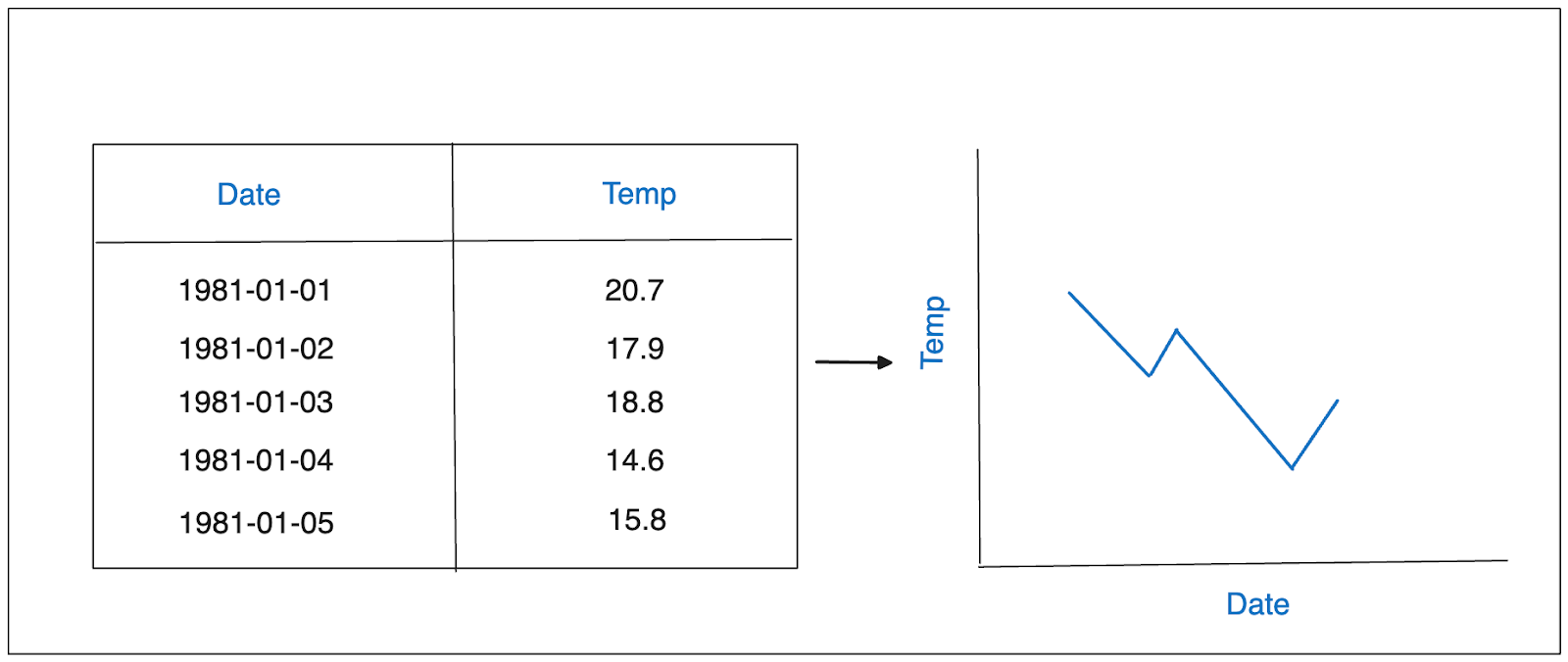
Time series data consists of data points recorded at regular (metrics) and irregular (events) time intervals and arranged chronologically. A defining feature of time series data is that each data point is associated with a specific timestamp, as illustrated in the following visualization:

Example of time series data.png

You’ve most likely encountered these kinds of data in your daily life, such as hourly weather temperature, daily website traffic over a month, sensor data recording wind turbine blade rotations per minute, monthly sales figures for a retail store over the past year, etc. People use time series data to gain insights about past patterns to drive strategic decisions in the future.

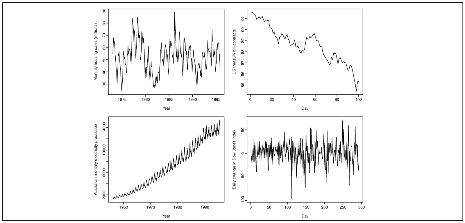
When dealing with time series data, you will typically find one or more of these patterns: seasonal, trend, or cyclic.

Seasonal refers to a fluctuating pattern in the data at a fixed frequency due to seasonal factors, such as the day of the week or the month of the year. Trend refers to a long-term decrease or increase in the data. Meanwhile, cyclic refers to a fluctuating pattern in the data, similar to seasonal, but without a fixed frequency.

Top left-seasonal top right-decreasing trend bottom left- increasing trend bottom right- cyclic.png

There are two types of time series data:

Univariate time series data: This involves a single time-dependent variable observed over successive time intervals. The daily weather temperature and stock price are two of the univariate time series examples.
Multivariate time series data: This involves multiple time-dependent variables recorded over the same time intervals. As an example, in addition to recording the weather temperature, other factors such as humidity and wind speed can also be recorded.

One traditional statistical approach for understanding linear dependencies and trends in time series data is the autoregressive integrated moving average (ARIMA) model.

Understanding Time Series Forecasting for Future Values

Time series forecasting involves predicting the future values of a time-dependent variable within a time series dataset. For example, if you have the historical price of a cryptocurrency for the past two years, you may want to predict its price a week from now.

Time series forecasting is not just a theoretical concept but a practical tool used by various companies across different sectors in their daily operations:

Financial Institutions: Banks and investment firms use time series forecasting to predict stock market trends, currency fluctuations, and detect anomalies in customer spending patterns. This helps in developing risk management strategies.
Healthcare Sector: Hospitals and healthcare providers utilize time series analysis to forecast patient admission rates, track the spread of diseases, and monitor patients’ vital signs. This powerful tool plays a crucial role in enhancing patient care and outcomes.
Retail Industry: Retailers leverage time series forecasting to predict sales volumes, analyze customer buying behavior, and efficiently manage inventory levels. This helps minimize stockouts, optimize pricing strategies, and enhance overall profitability.
Internet of Things (IoT): The Internet of Things (IoT) refers to billions of connected devices constantly creating and sharing data. We see this in smart homes, where devices like thermostats and home hubs exchange sensor data to automate tasks like adjusting temperatures or turning off lights when no one’s home. This interconnected network of sensors highlights the importance of time series analysis for IoT data.
Manufacturing: Manufacturers collect and analyze time-stamped data to reduce machine downtime that hurts the bottom line by adopting and improving predictive maintenance strategies.

We can use several models to conduct time series forecasting. In general, time series forecasting models fall into three categories: statistical, machine learning, and deep learning

Categories of time series forecasting model..png

Statistical models use traditional statistical methods for forecasting. Examples of models in this category include ARIMA, SARIMA, Exponential Smoothing, and Vector Autoregression. While statistical models are simple and effective in capturing basic trends and seasonality in univariate time series data, they may struggle with high-dimensional data with complex and non-linear patterns. Also, most statistical models only work with univariate data, and we need to look for another method if we have multivariate data.

Machine learning models often outperform statistical models, especially when dealing with high-dimensional time series data with complex and non-linear patterns. Examples of models in this category include Linear Regression, Random Forest, Gradient Boosting, and other regression algorithms. Determining the optimal value for parameters such as the time delay and hidden dimensions in a biLSTM architecture is critical for achieving the best performance and minimizing overfitting during training.

One advantage of machine learning models is their ability to incorporate exogenous data. Exogenous data refers to variables unrelated to the variable being forecasted. For example, when forecasting weather temperature, exogenous data could include humidity, wind speed, and days of the week. Integrating exogenous data can significantly enhance the predictive power of the model.

Since the inception of Transformers architecture, the advancement of time series forecasting with deep learning is also rapidly evolving. Examples of models in this category include LSTM, Informer, and Spacetimeformer. For huge time series data with complex and non-linear relationships, deep learning models may offer superior performance compared to machine learning and statistical models. Identifying the optimal values for certain parameters within algorithms is essential for enhancing performance and reducing errors, particularly in relation to chaos theory and time-series analysis.

However, one drawback of using deep learning models for time series forecasting is the lack of interpretability. The architecture of deep learning models are highly complex, meaning that we usually treat them as black boxes. This becomes problematic as interpretability is often crucial in time series forecasting.

In a univariate time series data with a simple pattern, we can take the data as it is and use statistical models to perform time series forecasting. However, we need to undertake additional preprocessing steps if we want to use more advanced methods like machine learning or deep learning on complex univariate or multivariate data.

Machine learning models expect the data to be structured in the form of a matrix, where each row represents one observation, and each column represents the features.

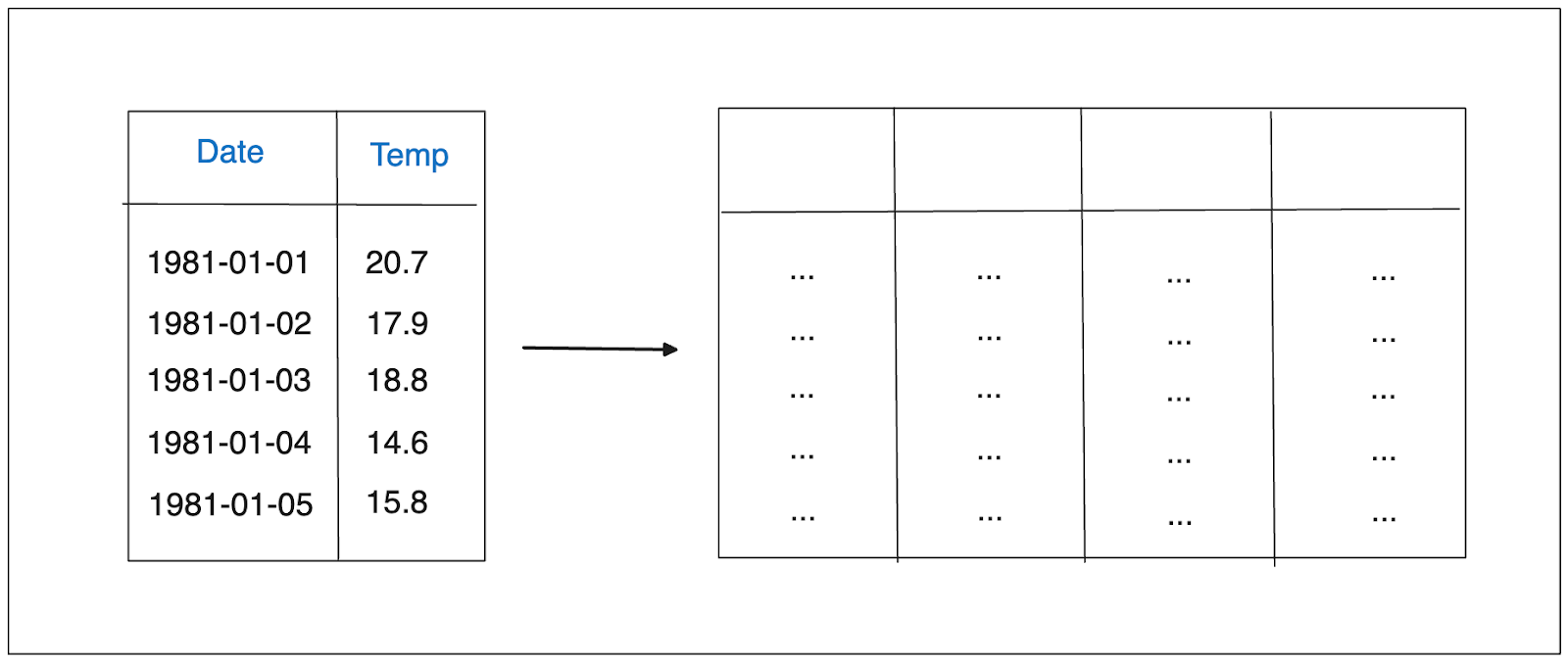Illustration of time series embedding..png

The question now is: how do we convert our time series data into a matrix form that is expected by our machine learning model? There are several methods we can use, such as using lag features, window features, or adding exogenous features.

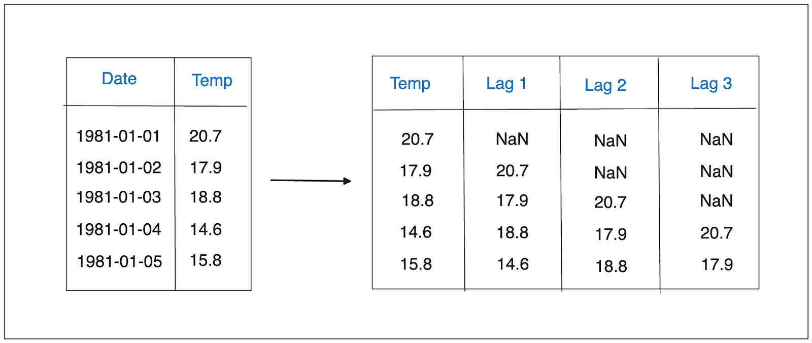
The concept of lag features is quite simple: we take the observation from n previous time steps and include them as features. In other words, we shift the data by n number of time steps, where n is the lag value that we can set in advance.

As an example, let’s say we set the lag values to be 1, 2, and 3. If we have a daily temperature data as shown below, then the transformation of the data would look something like this:

Lag features..png

In the visualization above, t-1 represents the temperature one day before the current temperature, t-2 represents the temperature two days before the current temperature, and t-3 represents the temperature three days before the current temperature. Adding lag features as preprocessing steps is necessary for our machine learning model as they provide insight into patterns of our time series data.

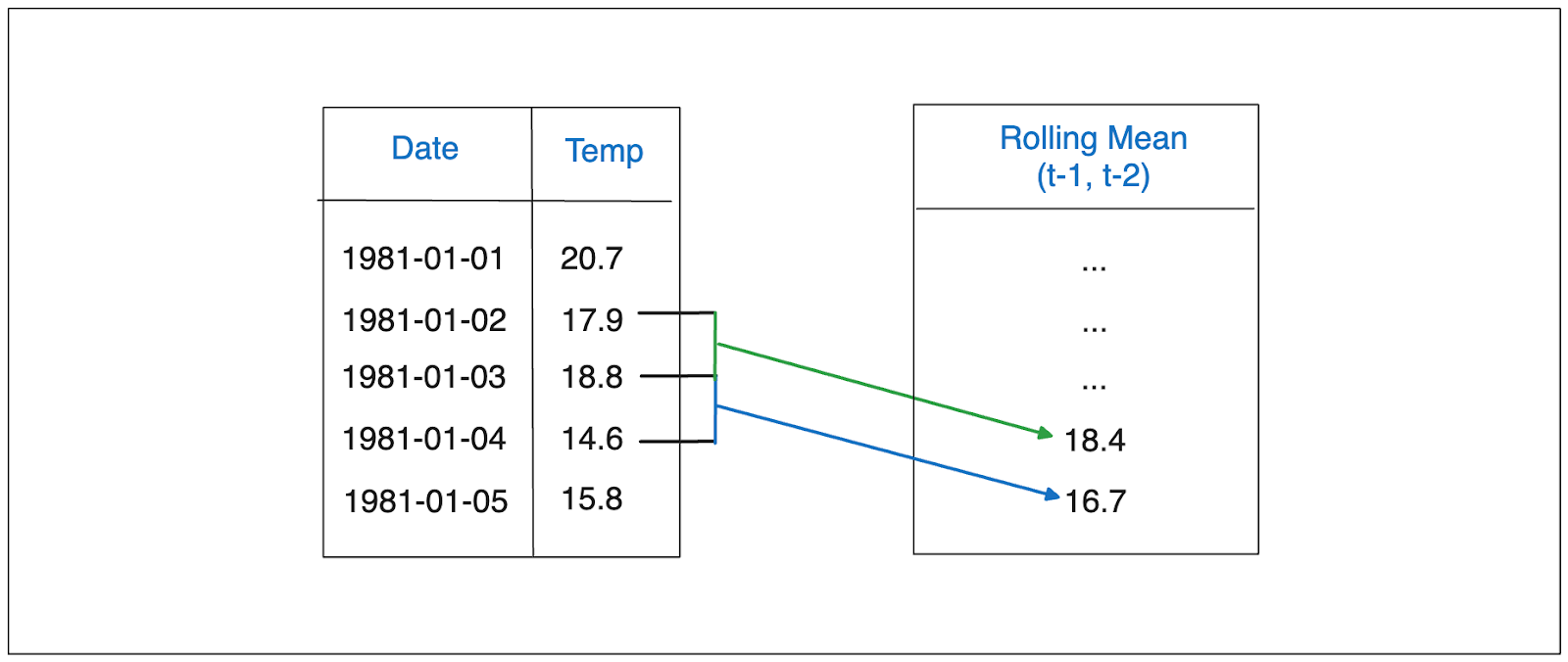
In addition to lag features, we can also transform our time series data into a matrix by using the summary statistics of a collection of previous n observations and including them as features. The summary statistics can be anything, such as the mean or median. However, the mean value is the popular choice for window features.

As an example, let’s say we want to implement window features on our daily temperature data, and we set the window value to be 2. In this case, we’ll use the mean of the previous two days as part of the features to predict today’s temperature.

Window features..png

Window features play an important role for our machine learning model during training as they provide insights into the local trends and fluctuations of our time series data. These features are very useful in cases where our time series data is non-stationary.

An exogenous feature refers to a feature that is not directly related to the variable we want to predict. In the context of temperature data, exogenous features can include the day of the week, humidity, wind speed, quarter of the year, etc.

However, we need to be careful when incorporating exogenous features. When we want to forecast the value of a variable at a particular time step, the value of all features should be known at that point. If we have features such as humidity and wind speed, we might not have the value of these features at the time of prediction.

Thus, as a rule of thumb, always ask yourself this question: would you have the information regarding the value of a feature by the time you need to make the forecast? If yes, you can add this feature as part of your time series embedding.

In this section, we’re going to implement a time series forecasting task. Along the way, we’ll transform our data into embeddings using all of the techniques mentioned in the previous section.

For the dataset, we'll use the minimum daily temperature data recorded in Melbourne, Australia, spanning over 10 years from 1981 to 1990. To transform the data into embeddings and train a regression model, we can utilize a popular machine learning library like scikit-learn. Let's load all the necessary libraries and the data.

import numpy as np
import matplotlib.pyplot as plt
import pandas as pd

from sklearn.ensemble import RandomForestRegressor
from sklearn.linear_model import Lasso
from sklearn.metrics import mean_squared_error

# Minimum daily temperature data
url = "<https://raw.githubusercontent.com/jbrownlee/Datasets/master/daily-min-temperatures.csv>"
df = pd.read_csv(url)

df["Date"] = df["Date"].apply(lambda x: pd.to_datetime(x))
df = df.set_index("Date")
df.head()

Input data..png

We have univariate weather temperature data recorded from 1981 to 1990. However, we can't use this data as it is if we want to train a machine learning model for a forecasting task. We need to transform the data into embeddings to capture any trends or seasonality in the data and to improve the performance of our model.

Let's implement a combination of lag, window, and exogenous features to embed the data. For lag features, we're going to set the lag values to be 1 and 7. For window features, we're going to compute the mean and standard deviation of the temperatures from the previous 14 days. For exogenous features, we're going to record the month, the year, and the quarter. After that, we'll drop all rows with null values.

# Lag features, set value to 1 and 7
df[f"y_lag_1"] = df["Temp"].shift(periods=1)
df[f"y_lag_7"] = df["Temp"].shift(periods=7)

# Window features, set the value to 14
result = (
    df["Temp"]
    .rolling(window=14) 
    .agg(["mean", "std"]) 
    .shift(periods=1) 
)  

result = result.add_prefix("y_window_14")
df = df.merge(result, how="left", left_index=True, right_index=True)

# Exogenous features, fetch month, year, and quarter
df["month"] = df.index.month
df["year"] = df.index.year
df["quarter"] = df.index.quarter

# Drop null values
df.dropna(inplace=True)

# Set temperature as the label
y = df["Temp"]
X = df.drop("Temp", axis=1)

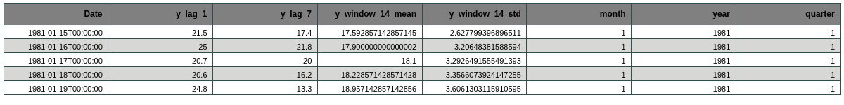Final feature embedding..png

And we've transformed our time series data into embeddings! Now we can use these embeddings as inputs to our regression model.

The final step before the training process is to split our data into a training set and a test set. To do this, we'll use the first 9 years of data as the training data and the last year as the test data. Then, we'll instantiate our regression model and train it using the training data.

end_train ='1990-01-01'

X_train = X.loc[:end_train]
X_test  = X.loc[end_train:]

y_train = y.loc[:end_train]
y_test  = y.loc[end_train:]

# Instantiate model and train it
lasso = Lasso(random_state=9)
lasso.fit(X_train, y_train)

Now that we have trained our model, we can perform time series forecasting with it on the test data and compare the forecasting result with the actual temperature value. Below is the data visualization of the forecasting result.

# Temperature forecasting on test data
preds = lasso.predict(X_test)
preds = pd.Series(preds, index=X_test.index)

# Plot forecasting results vs actuals
fig, ax = plt.subplots(figsize=(12, 8))
y_train[-200:].plot(ax=ax, label='train')
y_test[:200].plot(ax=ax, label='test')
preds.iloc[:200].plot(ax=ax, label='predictions')
ax.legend(bbox_to_anchor=(1.3, 1.0))

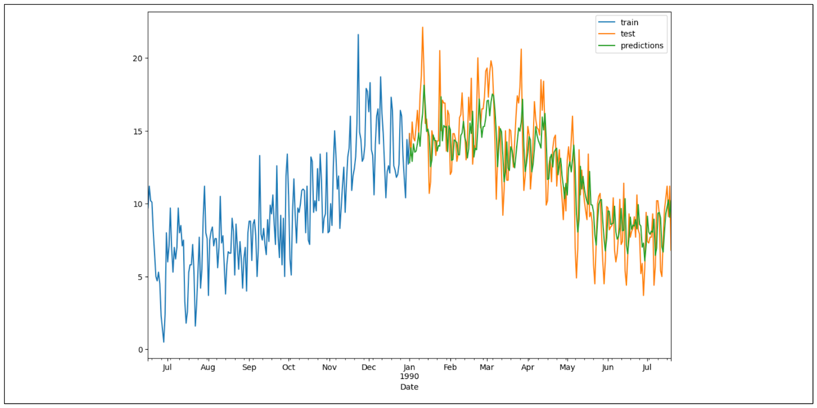Time series forecasting result..png

As you can see, our model’s forecasting results are quite good, as it can capture the trend and seasonality in our test data. You can experiment with the lag, window, and exogenous features to fine-tune the performance of our machine learning model.

Time series data consists of a series of observations recorded over specific time intervals, and they can exhibit one or more of the following patterns: seasonal, trend, and cyclic. To forecast this data using advanced methods like machine learning, we need to transform it into embeddings by introducing lag, window, or exogenous features. These features play a crucial role in our machine learning model, as they can effectively capture the seasonal, trend, or cyclic nature of the time series data. It’s important to note that the values for each feature need to be meticulously fine-tuned, taking into account the unique characteristics of the data and the domain knowledge.

Time Series Embedding Techniques

Time series embedding techniques are essential for transforming raw time series data into a structured format that machine learning models can process effectively. These techniques help in extracting meaningful features from the input data, enabling the models to capture underlying patterns and trends. Here are some common time series embedding techniques:

Lag Features: This technique involves taking observations from previous time steps and including them as features in the dataset. For instance, if we set a lag value of 3, the data point at time t will include the values from time t-1, t-2, and t-3 as additional features. Lag features are particularly useful for capturing recurring patterns and dependencies in the data.
Window Features: Window features involve calculating summary statistics, such as the mean or standard deviation, over a specified window of previous observations. For example, a window size of 5 would mean computing the mean of the last five data points and using it as a feature. This technique helps in capturing local trends and smoothing out short-term fluctuations in the data.
Exogenous Features: These are external variables that are not directly related to the target variable but can influence its behavior. For example, when forecasting sales, exogenous features could include holidays, promotions, or economic indicators. Incorporating exogenous features can significantly enhance the predictive power of machine learning models by providing additional context.
Autoencoders: Autoencoders are a type of neural network used to learn a compressed representation of the input data. They consist of an encoder that compresses the data and a decoder that reconstructs it. Autoencoders are effective in capturing complex, non-linear patterns in the data, making them suitable for high-dimensional time series.

By leveraging these time series embedding techniques, we can transform raw time series data into a format that is more suitable for machine learning models, ultimately improving their performance and accuracy.

Applications of Time Series Embedding

Time series embedding techniques have a wide range of applications across various fields, enabling organizations to gain insights and make data-driven decisions. Here are some key applications:

Time Series Forecasting: Embedding techniques are crucial for time series forecasting tasks, as they help in extracting relevant features from historical data. These features can then be used to train machine learning models to predict future values. For example, retailers can forecast future sales by embedding past sales data along with exogenous features like holidays and promotions.
Anomaly Detection: By transforming time series data into embeddings, machine learning models can identify unusual patterns or outliers. For instance, in the healthcare sector, embedding techniques can help detect anomalies in patient vital signs, enabling early intervention and improving patient outcomes.
Clustering: Time series embedding techniques can be used to group similar time series data together. This is useful in various applications, such as segmenting customers based on their purchasing behavior or grouping similar sensor readings in IoT applications. Clustering helps in identifying common patterns and trends across different time series.
Classification: Embedding techniques can also be used for classifying time series data into different categories. For example, in natural language processing, time series embeddings can help classify text data based on sentiment or topic. By analyzing the embedded data, machine learning models can accurately identify patterns that distinguish different classes.

These applications demonstrate the versatility and importance of time series embedding techniques in various domains, enabling organizations to leverage machine learning models for better decision-making.

Best Practices for Time Series Embedding

Implementing time series embedding techniques effectively requires careful consideration of several factors. Here are some best practices to ensure optimal results:

Choose the Right Technique: The choice of embedding technique should align with the specific problem you are addressing. For instance, lag features are ideal for capturing short-term dependencies, while window features are better suited for identifying long-term trends. Understanding the nature of your data and the problem at hand will guide you in selecting the most appropriate technique.
Select Relevant Features: Including irrelevant features can degrade the performance of your machine learning model. Focus on selecting features that have a meaningful relationship with the target variable. For example, when forecasting weather, features like humidity and wind speed are relevant, while unrelated features should be excluded.
Optimize Hyperparameters: Hyperparameters such as the embedding dimension and time delay can significantly impact the performance of your model. Experiment with different values to find the optimal embedding dimension and other hyperparameters that yield the best results. Tools like grid search or random search can help in this optimization process.
Use Domain Knowledge: Leveraging domain knowledge can enhance the effectiveness of your embeddings. For example, understanding seasonal factors in sales data can help in selecting relevant features and setting appropriate lag or window values. Domain expertise can provide valuable insights that improve the quality of your embeddings.
Evaluate Performance: Regularly evaluate the performance of your machine learning model using metrics such as mean absolute error (MAE) and root mean squared error (RMSE). These metrics help in assessing the accuracy of your forecasts and identifying areas for improvement. Continuous evaluation ensures that your model remains robust and reliable.

By following these best practices, you can effectively implement time series embedding techniques, leading to more accurate and reliable machine learning models.

Ruben Winastwan

Next: Enhancing Information Retrieval with Learned Sparse Retrieval

Content

Start Free, Scale Easily

Try the fully-managed vector database built for your GenAI applications.

Try Zilliz Cloud for Free