Streamlining Data: Effective Strategies for Reducing Dimensionality
In this article, we'll discuss how having too much data can hinder the performance of our machine-learning model and what we can do to address this problem.
Read the entire series
- Natural Language Processing Fundamentals: Tokens, N-Grams, and Bag-of-Words Models
- Primer on Neural Networks and Embeddings for Language Models
- Sparse and Dense Embeddings
- Sentence Transformers for Long-Form Text
- Training Your Own Text Embedding Model
- Evaluating Your Embedding Model
- Class Activation Mapping (CAM): Better Interpretability in Deep Learning Models
- CLIP Object Detection: Merging AI Vision with Language Understanding
- Discover SPLADE: Revolutionizing Sparse Data Processing
- Exploring BERTopic: A New Era of Neural Topic Modeling
- Streamlining Data: Effective Strategies for Reducing Dimensionality
- All-Mpnet-Base-V2: Enhancing Sentence Embedding with AI
- Time Series Embedding in Data Analysis
- Enhancing Information Retrieval with Learned Sparse Retrieval
- What is BERT (Bidirectional Encoder Representations from Transformers)?
- What is Mixture of Experts (MoE)?
If you’re a data science practitioner, you might have heard the rule of thumb for training a machine learning model: the more data you have, the better the model's performance will be. However, this rule might not hold true in all scenarios.
In this article, we'll explore this issue, discussing how having too much data can hinder the performance of our machine-learning model and what we can do to address this problem.
So, without further ado, let's dive in!
The Curse of Dimensionality
Before we discuss the challenges of having too much data, it's important to understand the concept of dimensions.
In data science, dimensions refer to the number of input variables or features in a dataset. For instance, in a housing dataset, dimensions might include the house price, number of bedrooms, number of bathrooms, floor area, address, year built, and facilities inside.
You might assume that adding more dimensions to our machine-learning model would enhance its performance. However, the opposite is often true. This is because the more we increase the dimensions of our data, the sparser it becomes. Imagine a line (1D) – filling that space with a few data points is relatively easy. With a rectangle (2D), we need more data points to cover its area. If we consider a cube (3D), even more data points are required to fill it.
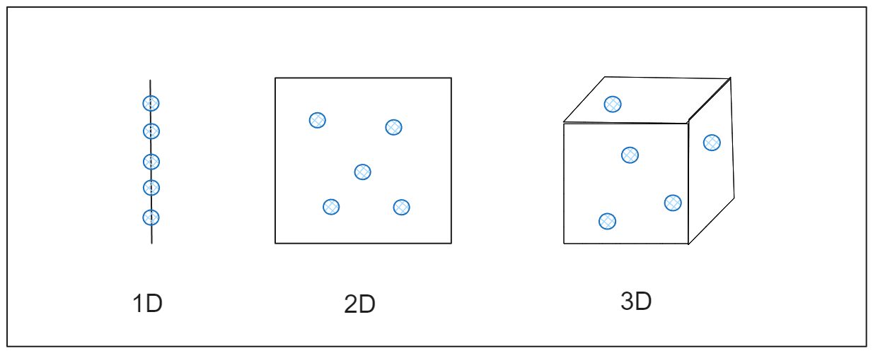 Image by author
We can call the space that our data needs to fill in a n-dimensional space as a feature space. A higher dimensionality means a larger feature space, necessitating more data points to extract meaningful information from our data.
Higher dimensionality leads to several problems:
Computational resources: More dimensions require increased computational resources for data processing.
Data sparsity: As the feature space expands, data points will likely be more dispersed, complicating machine learning models' clustering and classification tasks.
Model performance degradation: A larger feature space can reduce performance for algorithms that rely on distance metrics, such as KNN or k-means clustering. Moreover, excessive dimensions can lead to overfitting, where the model fits too closely to the data and struggles to generalize to unseen data points.
Visualization difficulty: High-dimensional data are challenging to visualize, making it harder to analyze and interpret.
The problems mentioned above are what people call “the curse of dimensionality.”
So, how can we mitigate the curse of dimensionality and obtain the intrinsic dimensionality of our data? There are several methods to address this problem, and we'll explore them in the next section.
Dimensionality Reduction Algorithms
To address the curse of the dimensionality problem, several common dimensionality reduction techniques are applied in data science. These algorithms include Principal Component Analysis (PCA), t-Distributed Stochastic Neighbor Embedding (t-SNE), and Uniform Manifold Approximation and Projection (UMAP).
Principal Component Analysis (PCA)
PCA is perhaps one of the most well-known dimensionality reduction techniques available. In essence, PCA projects data onto axes that preserve the maximum variance. But what does this mean? Consider the following example of data points in a 2D feature space.
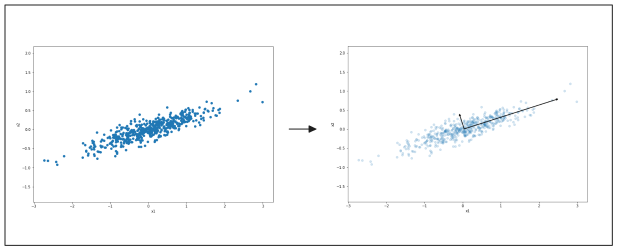 Image by author
left: 2D scatter plot, right: principal components of PCA
PCA, a crucial tool in data analysis and machine learning, can be used to reduce the dimensionality to 1D (a line). First, PCA seeks to find the axis that preserves the most information from our data points, ensuring we keep significant information when projecting the data into 1D. As you can see from the visualization on the right-hand side above, the longer vector represents the projection that retains the most information from our data compared to the shorter vector.
PCA selects the projection that preserves the most information. Thus, it chooses the longer vector as the first axis. Next, it identifies the second axis, which is orthogonal to the first projection and preserves the second most information from our data.
In our 2D feature space example above, the second axis would align with the shorter vector in the visualization above. PCA will also identify the third axis if we have a 3D or higher-dimensional feature space.
The axes selected by the PCA algorithm are known as the principal components. Once all principal components have been determined, PCA projects our feature space into a lower dimension, as illustrated below.
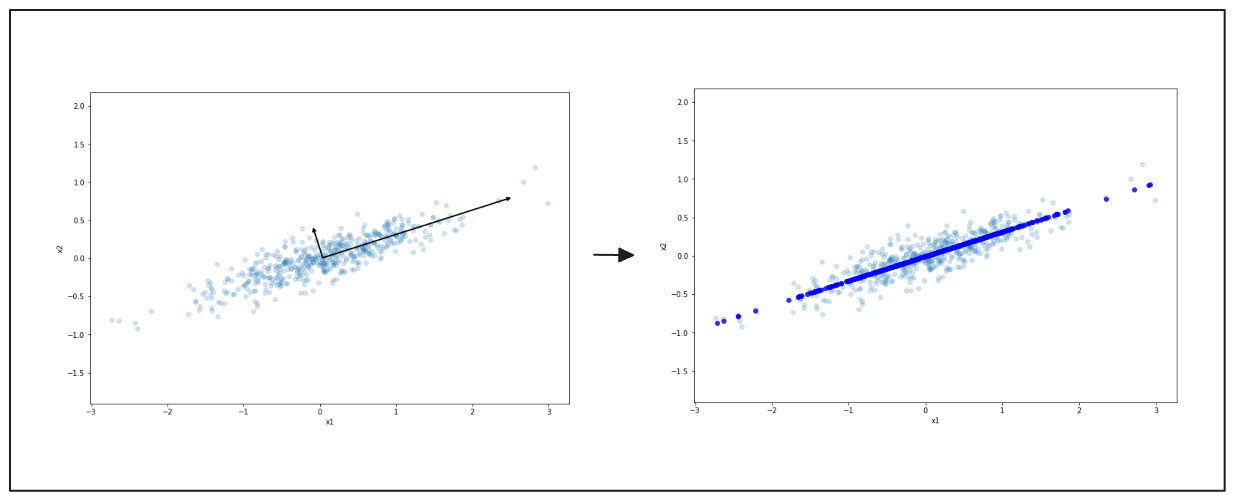 Image by author
left: principal components of PCA, right: final projection result from PCA, visualized with dark blue line
t-distributed Stochastic Neighbor Embedding (t-SNE)
PCA might not produce good results when dealing with datasets that contain non-linearly separable data points. Consider a Swiss roll dataset in 3D space, as shown in the visualization below. The data points from different classes are scattered throughout the feature space. In such cases, linear PCA may not provide a meaningful projection, as illustrated on the right-hand side of the image below.
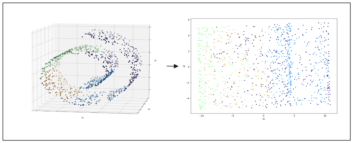 Image by author
left: swiss roll 3D data points, right: 2D projection result from PCA
Projection-based algorithms may not be the best solution when dealing with non-linearly separable data points. This is where manifold-based algorithms like t-SNE come into play.
t-SNE is an improvement of the original SNE algorithm, first introduced in 2002. The 't' in t-SNE indicates that it uses a t-distribution instead of a normal Gaussian distribution to compute the similarity between each data point in the lower-dimensional space.
One characteristic of the t-distribution is that it has heavier tails than the Gaussian distribution. This feature enables the t-SNE algorithm to visualize different clusters at sparser distances.
Let's say we have data points scattered across a 2D feature space, and we want to reduce its dimensionality to 1D.
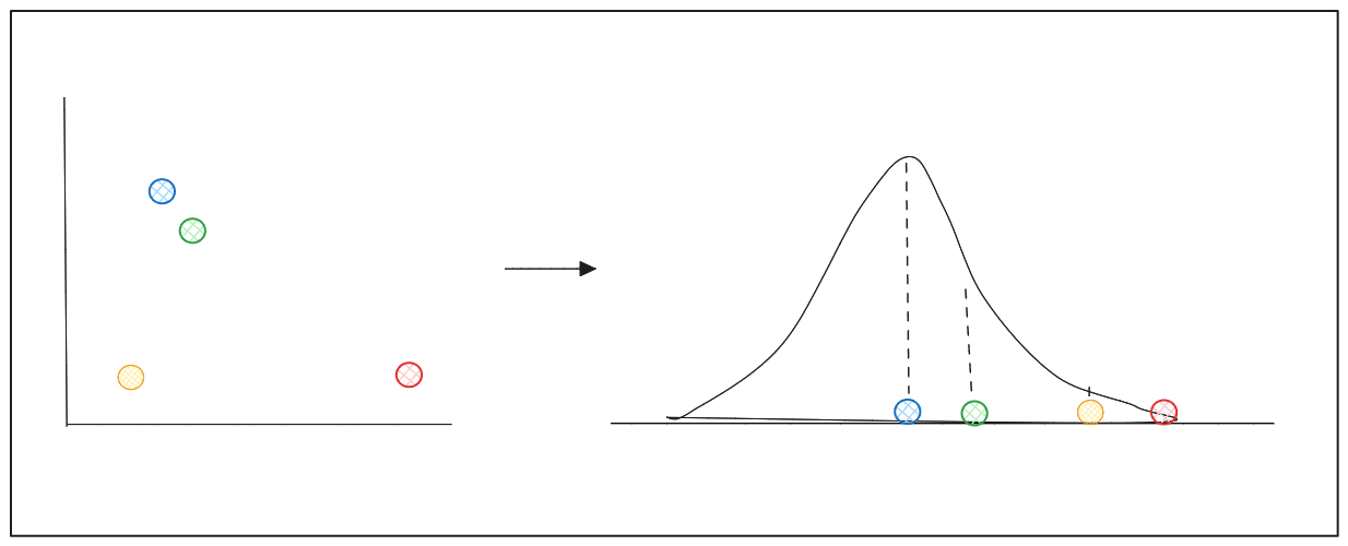 Image by author
left: 2D scatter points, right: distribution centered around a data point to find similarity of neighboring points
For each data point xi, the algorithm estimates the similarity of each neighbor xj using a Gaussian distribution centered around xi. The outcome of this step is the probability of each neighbor, which we refer to as Pij.
The variance of the Gaussian distribution around xi depends on the density of data points near xi. This parameter is often referred to as perplexity in t-SNE. The higher the density around a data point, the higher the perplexity value. Given the varying density around each data point, we may obtain distributions with different variances for different data points.
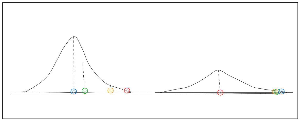 Image by author (distributions with different variance.png)
Due to the diversity of densities, the algorithm normalizes the similarity between xi and its neighbors so that the total similarity adds up to 1.
In the next step, the algorithm aims to find a probability in the lower-dimensional space, Qij, closely resembling Pij. To measure the similarity between Pij and Qij, t-SNE uses the Kullback-Leibler (KL) divergence, represented by the following equation:
This KL divergence equation is optimized using a gradient descent algorithm, similar to the one used to optimize regression algorithms.
Uniform Manifold Approximation and Projection (UMAP)
While t-SNE generally excels at handling complex data points, the computational resources required to execute this algorithm can be quite high, especially with a large dataset. This is due to the necessity of calculating each data point's pairwise similarity. UMAP is a viable alternative to t-SNE for managing non-linearly separable and complex data points.
At a high level, UMAP operates similarly to t-SNE. It transforms the data's high-dimensional representation into its lower-dimensional counterpart using an optimization technique.
UMAP uses a graph-based algorithm to identify the data structure in high-dimensional space. Specifically, it utilizes a fuzzy simplicial complex algorithm. If you’re familiar with graph algorithms, this is essentially a graph with weighted edges. The weight indicates the likelihood that two data points are connected.
Consider a 2D scatter plot as shown below:
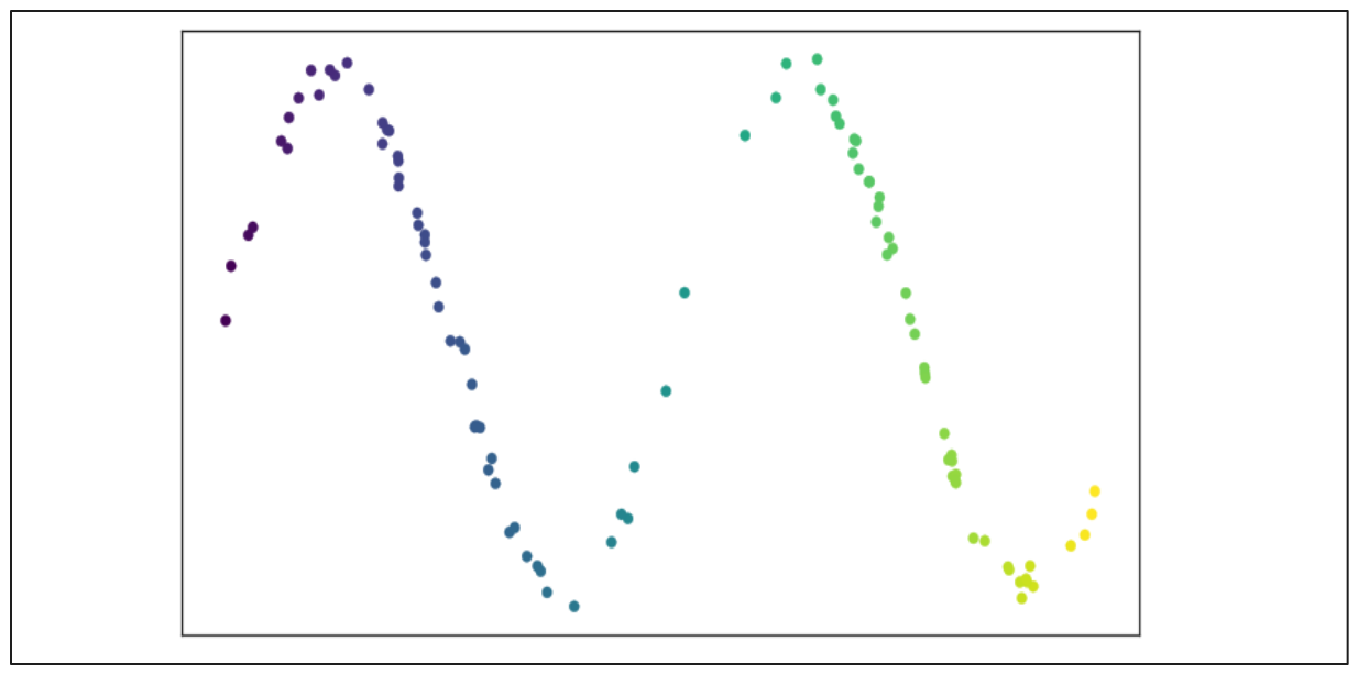
Image source: UMAP documentation
To construct the graph from these data points, we first specify the nearest neighboring points (n) each data point should consider. Then, UMAP extends a radius outward from each point based on the distance to the n-th nearest neighbor. A data point will be connected to its neighbor if their radii overlap.
However, the likelihood of connection (edge weight) decreases as the radius expands. This method ensures that each data point is connected to at least one of its closest neighbors. It maintains a balance between the global structure in higher-dimensional space and the local structure in lower-dimensional space.
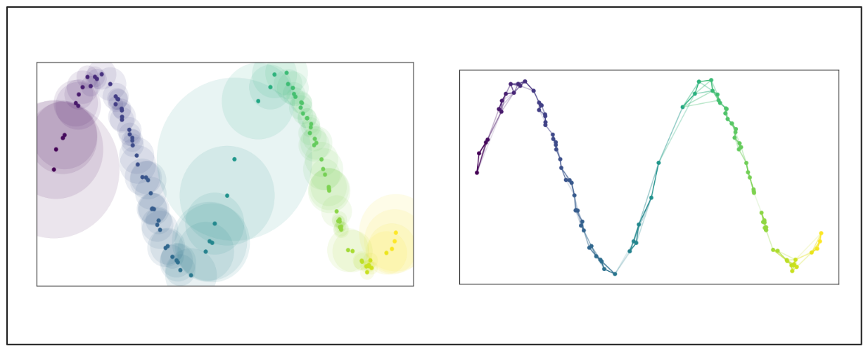
Image source: UMAP documentation
Once the graph in high-dimensional space is constructed, the algorithm aims to replicate this layout in the low-dimensional space to be as similar as possible via an optimization function similar to t-SNE.
One of the most prominent differences between UMAP and t-SNE is the balance between global and local structure. In most cases, UMAP is better at preserving the global structure of the data in the final projection in lower dimensional space. This means that the inter-cluster relations are more meaningful than in t-SNE.
Implementation of Dimensionality Reduction
In this section, we'll perform dimensionality reduction on the MNIST handwritten digits dataset using all three algorithms we discussed in the previous section. To do so, we'll utilize the popular machine learning library, Scikit-learn. Let's first load the handwritten digits data.
| !pip install umap-learn import seaborn as sns from umap import UMAP from sklearn.decomposition import PCA from sklearn.manifold import TSNE from sklearn.datasets import fetch_openml sns.set(style='white', rc={'figure.figsize':(12,8)}) # Fetch data mnist = fetch_openml('mnist_784') data = mnist.data labels = mnist.target |
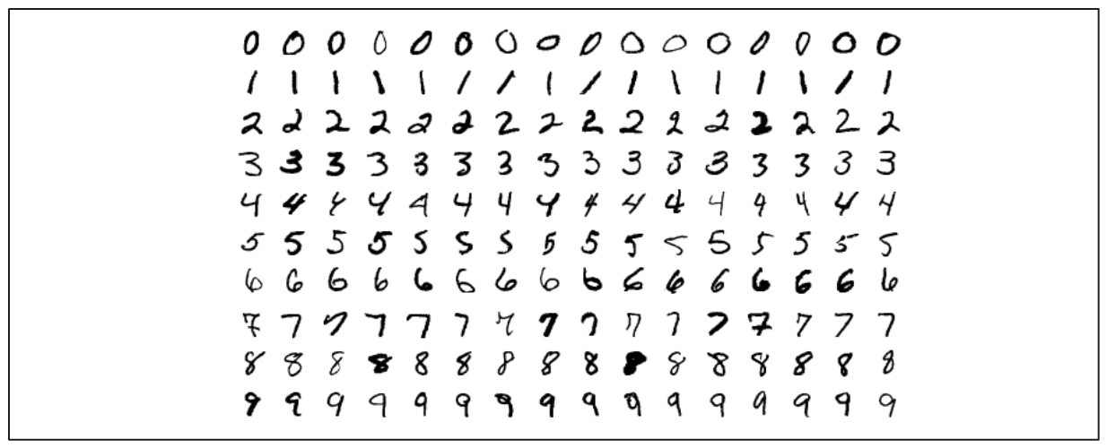
Image source: Wikipedia
Our dataset consists of images of handwritten digits ranging from 0 to 9, totaling 70,000 images. Each image is a flattened version of a 28 x 28-pixel matrix, resulting in 784 dimensions. Therefore, the shape of our data is (70,000, 784).
We can initialize PCA and t-SNE using the Scikit-learn library, while for UMAP, we need to initialize from a standalone library built based on Scikit-learn. We’ll use the library’s default values as the parameters for each algorithm. Next, we'll fit each algorithm with our data and apply dimensionality reduction.
| embeddings = { "PCA embedding": PCA( n_components=2, random_state=0 ), "t-SNE embedding": TSNE( n_components=2, random_state=0 ), "UMAP embedding": UMAP( n_components=2, random_state=0 ) } projections = {} for name, transformer in embeddings.items(): print(f'Computing {name}...') projections[name] = transformer.fit_transform(data) |
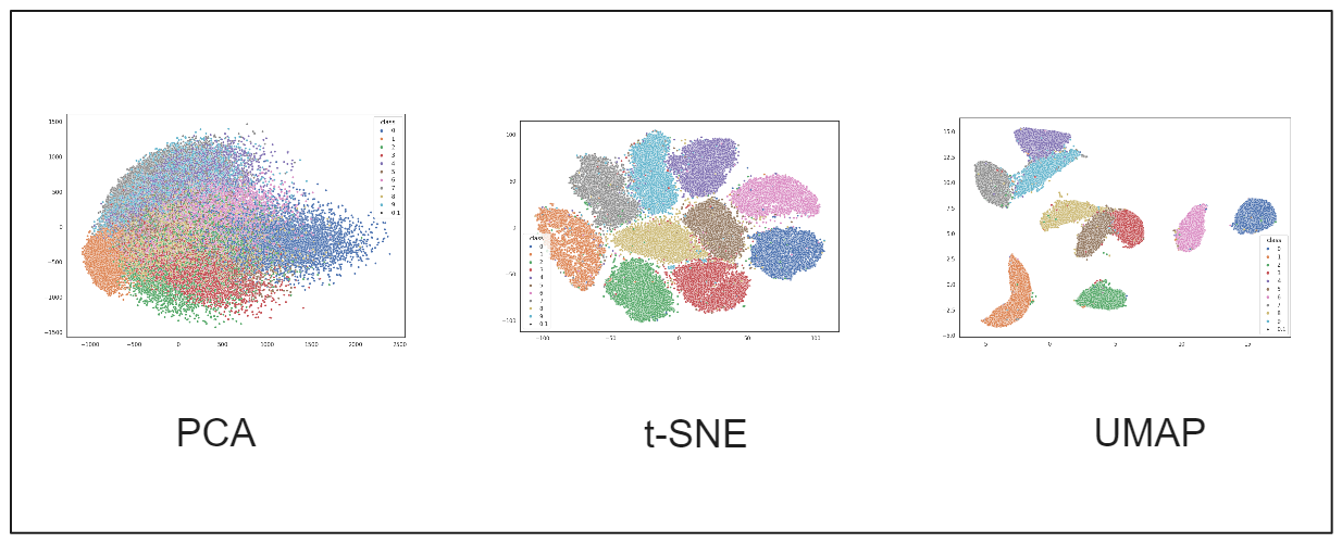 Image by author
As you can see from the visualization above, PCA's dimensionality reduction is insufficient to capture meaningful information from our data. This is understandable since PCA is a projection algorithm that performs best when the data is linearly separable. The first few principal components can explain the variance of the data. However, this is not the case for our MNIST dataset.
On the other hand, the results from both t-SNE and UMAP are pretty good. We can observe distinct clusters formed by data points belonging to different classes. The clusters formed by UMAP are slightly better than those by t-SNE, with fewer digits placed in incorrect clusters. From a runtime perspective, UMAP also outperforms t-SNE, as t-SNE's computational complexity increases as the number of data points grows.
Applications of Dimensionality Reduction Algorithm
In addition to being highly useful for data visualization, all of the dimensionality reduction algorithms discussed in this article offer various benefits across different use cases:
Natural Language Processing (NLP) tasks: These algorithms can visualize word embeddings from a large text corpus, making it easier to identify semantically similar words.
Clustering and Classification Tasks: They can help create segments or clusters of data points in a lower-dimensional space, facilitating the identification of patterns and trends in the data.
Anomaly Detection: These algorithms can identify outliers in the data, enabling us to address them appropriately during our data analysis.
Computer Vision: They can assist in the compression of image or video data, leading to efficient data storage without losing important information.
Feature Selection and Feature Engineering: These algorithms can remove redundant features, improving machine learning model performance and interpretability.
Conclusion
Having too many features in our data can lead to the curse of dimensionality problem, where the feature space becomes excessively large. This introduces several issues, such as data sparsity, model performance degradation, and data interpretation difficulties. Dimensionality reduction algorithms address these problems by projecting the data onto a lower-dimensional space while preserving the global structure of the data.
PCA produces excellent results when our data points are linearly separable, and the first few principal components can explain the variance of the data. For more complex data points, t-SNE and UMAP are better choices. However, when dealing with many data points, UMAP is preferable due to its superior computational efficiency compared to t-SNE.
We hope this article helps you get started with the concept of dimensionality reduction. Happy learning!
- The Curse of Dimensionality
- Dimensionality Reduction Algorithms
- Implementation of Dimensionality Reduction
- Conclusion
Content
Start Free, Scale Easily
Try the fully-managed vector database built for your GenAI applications.
Try Zilliz Cloud for FreeKeep Reading

Primer on Neural Networks and Embeddings for Language Models
Exploring neural network language models, specifically recurrent neural networks, and taking a sneak peek at how embeddings are generated.

Training Your Own Text Embedding Model
Explore how to train your text embedding model using the `sentence-transformers` library and generate our training data by leveraging a pre-trained LLM.

What is Mixture of Experts (MoE)?
Mixture of Experts (MoE): a neural network architecture to improve model efficiency and scalability by selecting specialized experts for different tasks.


