Matryoshka Representation Learning Explained: The Method Behind OpenAI’s Efficient Text Embeddings
Developing real-life machine learning models always involves a trade-off between cost and performance. For example, the larger the model and dataset we use during training, the more capable our trained model will ultimately be. However, this increased capability comes with a longer time and higher computational costs, as training requires significantly longer durations. The same principle applies during inference, where larger models tend to generate bigger feature representations that require greater memory for storage.
Since the needs during machine learning training and inference can vary significantly from one use case to another, it is essential to have a method that allows us to trade off a small portion of a model's performance in exchange for reduced costs. This is where a method like Matryoshka Representation Learning (MRL) comes into play. For instance, OpenAI’s text-embedding-3-small model utilizes MRL to enable developers to shorten embeddings while maintaining their core concept-representing properties. By allowing the adjustment of embedding dimensions, MRL helps strike the perfect balance between cost efficiency and model performance.
This article will explore how MRL works, its implementation, and how it allows for scalable and efficient machine-learning models. Let’s start with the motivation behind MRL.
The Motivation Behind Matryoshka Representation Learning (MRL)
The cost-performance trade-off is always a consideration before developing or using any machine learning models.
During training, a model’s parameters and the amount of training data directly influence its final performance. Larger models and training datasets tend to result in more capable models. However, the computational cost to train these models is also higher.
Meanwhile, during inference, larger models produce bigger feature representations. This increase in feature representations means we need more memory to store them.
Let’s use BERT as an example in the context of information retrieval. BERT is one of the earliest Transformer-based deep learning models that achieved state-of-the-art performance on several benchmark datasets in text classification, Named Entity Recognition (NER), question answering (QnA), and more.
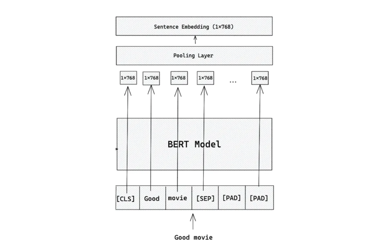
Figure: Workflow of embedding generation using BERT base model.
In a nutshell, BERT takes a sentence or a word as input and transforms it into a fixed-size embedding. This embedding captures the semantic meaning of the original input, and its size depends on the specific model variant used.
BERT has two main variants: the base model and the large model. The base model produces a 768-dimensional embedding, while the large model generates a 1024-dimensional embedding.
Let’s say we want to store 10 million embeddings in a vector database for an information retrieval use case. If we use the BERT base model in FP32 format, we’ll need roughly 768×10M×4=30.72 GB of memory to store these embeddings. In contrast, using the BERT large model in the same scenario would require around 40.9 GB. Additionally, a larger embedding size can slow down the retrieval process by increasing the computational complexity of similarity searches. However, the primary advantage of using larger embeddings is their enhanced ability to retrieve highly relevant information compared to smaller embeddings.
One ideal solution to these problems in information retrieval is splitting the whole process into two parts: shortlisting and reranking. Shortlisting refers to retrieving an initial set of candidate documents from a vast collection in our vector database like Milvus. Reranking then takes these shortlisted candidates and reorders them to maximize the relevance of the final results.
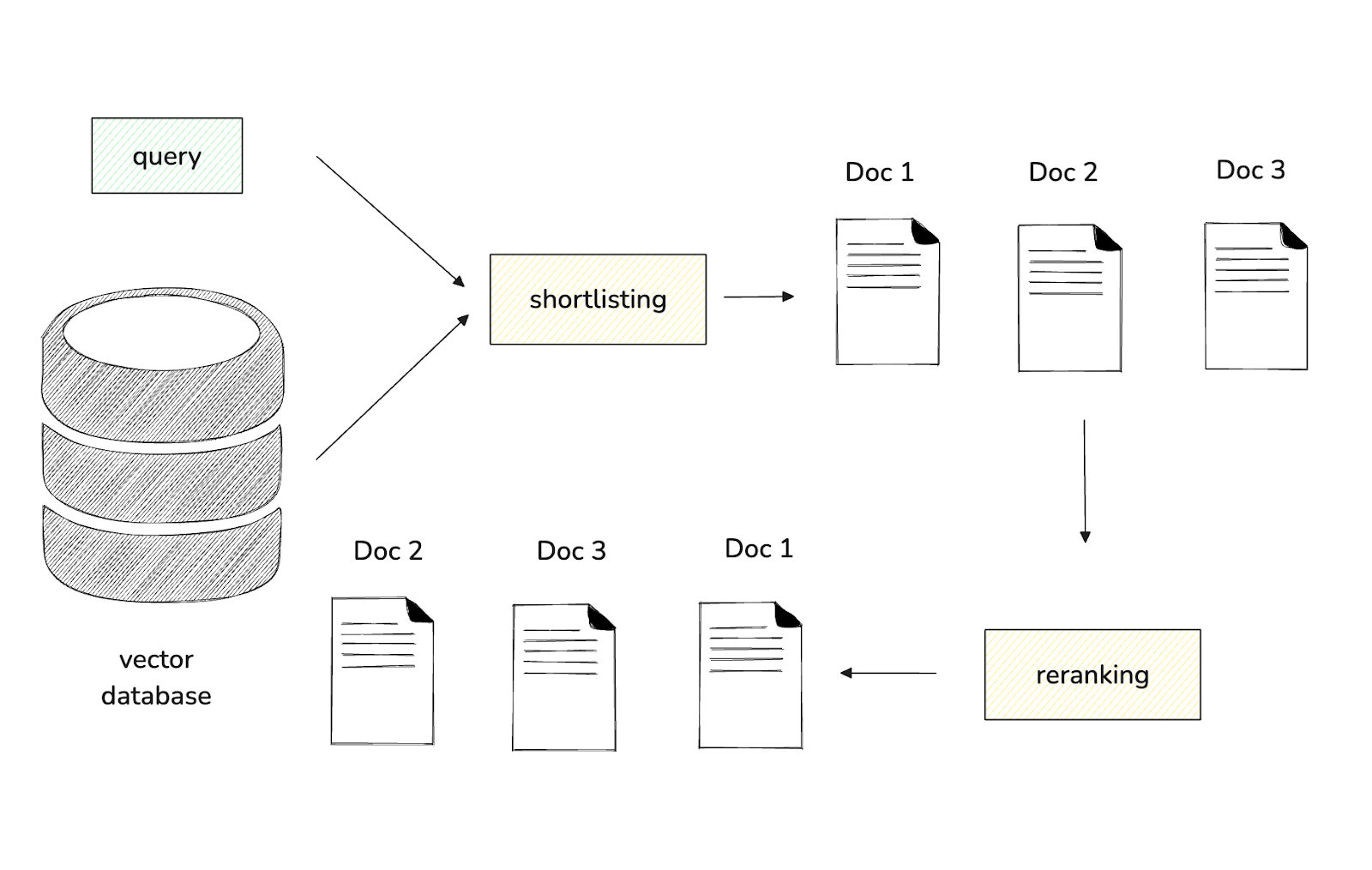 Figure- Shortlisting and reranking workflow
Figure: Shortlisting and reranking workflow.
To perform shortlisting, the algorithm computes the similarity between query embeddings and a large collection of embeddings stored in the vector database. Therefore, using smaller embedding sizes can make this computation more efficient and faster. Conversely, reranking emphasizes precision, which means we would benefit from larger embedding sizes.
The problem with this method is that once we select a particular model, the size of the embeddings or feature representations it produces is fixed. This lack of flexibility limits our ability to use embeddings of different sizes from a single model.
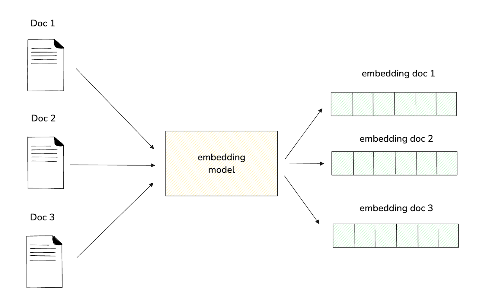 Figure- Workflow of a model generating a fixed-size embedding..png
Figure: Workflow of a model generating a fixed-size embedding.
The Matryoshka Representation Learning (MRL) approach offers an intriguing solution to this problem: models trained with this method can produce embeddings of various sizes. We will explore the mechanism of this approach in detail in the next section.
What is Matryoshka Representation Learning (MRL)?
Matryoshka Representation Learning (MRL) is a method for training neural networks to produce multi-scale representations within a single model. Inspired by Matryoshka dolls, where smaller dolls fit inside larger ones, MRL enables a model to output representations of varying sizes (from coarse to fine) using a single forward pass. This approach enables deep learning models to better understand complex relationships and nuances in data. MRL is particularly effective for tasks like semantic search, information retrieval, multilingual processing, and any application requiring nuanced representations of data across different levels of abstraction.
 Visualization of Matryoshka embeddings with multiple layers of detail
Figure: Visualization of Matryoshka embeddings with multiple layers of detail
Popular embedding models that have adopted the Matryoshka Representation Learning (MRL) approach include OpenAI’s text-embedding-3-large, Nomic’s nomic-embed-text-v1, and Alibaba’s gte-multilingual-base.
How the MRL Approach Works
The MRL approach enables us to extract feature representations from any machine learning model in several sizes. For example, instead of using the original 1024 dimensions of an embedding, we can utilize the first 16, 32, 64, 128, or 256 dimensions (or any dimensions we choose). The key to this capability lies in the way the model is trained when implementing the MRL approach.
 Figure- MRL loss function training and its use case during inference
Figure: MRL loss function training and its use case during inference. Source.
During model training with MRL, we optimize not just one loss function, as is typical in standard model training, but several. Each loss function aims to optimize the feature representation for a specific dimension that we define in advance. If we set five different feature dimensions, we will need to optimize five distinct loss functions during training.
Let’s say we want to train a BERT large model using the MRL approach. As mentioned in the previous section, this model generates an embedding of size 1024. If we set the feature dimensions to 32, 64, 128, 256, and 1024, we will optimize five different loss functions during training so that the model learns to generate optimized embeddings in those dimensions.
The optimization across these various dimensions is straightforward: MRL breaks down the overall loss function into the sum of losses for each individual dimension. Using our example above, this can be expressed as:

The optimization process for a model trained with MRL can be represented more formally as follows:

Figure: Optimization equation of MRL approach. Source.
As you can see, the definition of the loss function above is quite general. Therefore, the MRL approach can be applied to almost any model and is entirely independent of the model's architecture. We can also fine-tune pre-trained models like BERT or any other transformer-based models to output embeddings of various sizes. Continuing our scenario above, we can now generate 1024-dimensional embeddings from our trained BERT large model and 32, 64, 128, and 256-dimensional embeddings.
Overall, after training a model with MRL, the initial dimensions of the features generated by the trained model carry more significant information than later dimensions. The first few dimensions contain high-level details, while the later dimensions focus on more granular information, mimicking how a Matryoshka doll is structured.
However, this does not mean that shorter embeddings are always simply the truncated versions of longer ones. The values of each element in shorter embeddings might differ from those in longer embeddings from the scaling factor applied to each feature dimension during training. However, if we set the scaling factor in each dimension to be equal, the values of each element between shorter and longer embeddings might look identical.
MRL Experimental Results
The MRL approach has been evaluated on machine learning models across different modalities, including text, vision, and vision-text. ResNet50 and ViT models represent vision-based models, BERT represents text-based models, and ALIGN represents the combination of vision and text. These models have primarily been assessed for two common use cases: classification and retrieval. Let’s discuss classification first.
When comparing the performance of the ResNet50 model trained on the ImageNet-1K dataset to an independently trained standard ResNet50, the MRL model achieves comparable top-1 accuracy at various feature representation sizes.
To further gauge the utility of the feature representations for downstream tasks, the accuracy of 1-nearest neighbor (1-NN) for each size of feature representation was also measured. The setup for calculating 1-NN is as follows: given 1.3K image samples in the database, the task is to find the nearest neighbor for each of 50K queries. With this setup, the ResNet50 trained with MRL is up to 2% more accurate at each feature representation size compared to its fixed-feature counterpart.
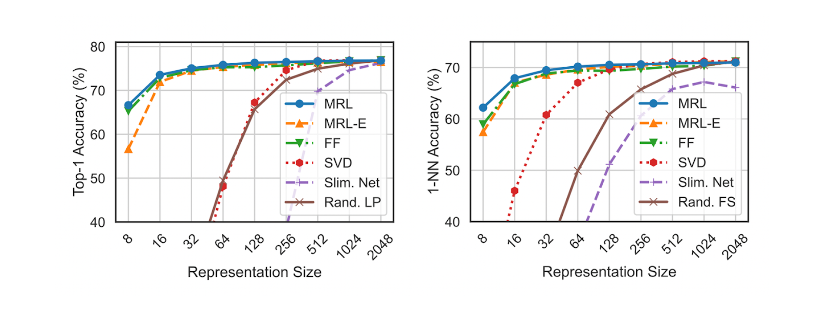 Figure- Top-1 accuracy and 1-NN accuracy of ResNet50 on ImageNet-1K
Figure: Top-1 accuracy and 1-NN accuracy of ResNet50 on ImageNet-1K. Source.
Meanwhile, the performance of the ViT model trained with MRL on the JFT-300M dataset is also very competitive across all representation sizes. Its 1-NN accuracy is comparable to that of ViT trained with fixed-size feature representations. As shown in the figure below, the performance of the MRL model is also better than its fixed-size counterpart at lower feature representations, partly because random features are selected from the fixed-size model to represent lower dimensions. A similar trend is observed with the ALIGN model trained using the MRL approach; its performance matches that of the ALIGN model trained with fixed-size representations.
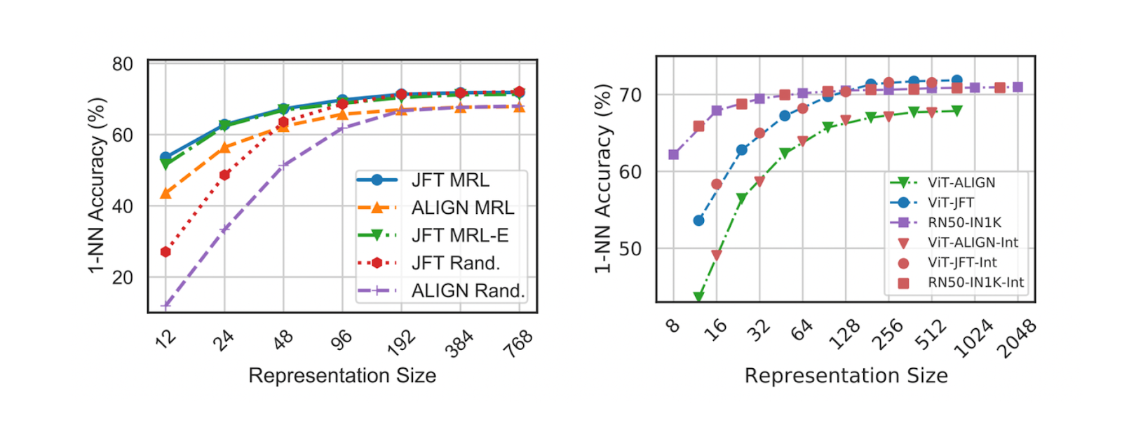 Figure- 1-NN accuracy of ViT and ALIGN on ImageNet-1K
Figure: 1-NN accuracy of ViT and ALIGN on ImageNet-1K. Source.
The main advantage of using the MRL approach is its flexibility to switch between different sizes of feature representations from the same model. To fully leverage this strength, tests on adaptive classification using ResNet50 on ImageNet-1K were also conducted.
This setup involves learning the maximum softmax probability to determine transitions from smaller feature representations to larger ones. The test results show that the MRL model with a 37-dimensional feature representation is as accurate as the ResNet50 model trained with a fixed 512-dimensional feature representation while being only 0.8% less accurate than the 2048-dimensional model.
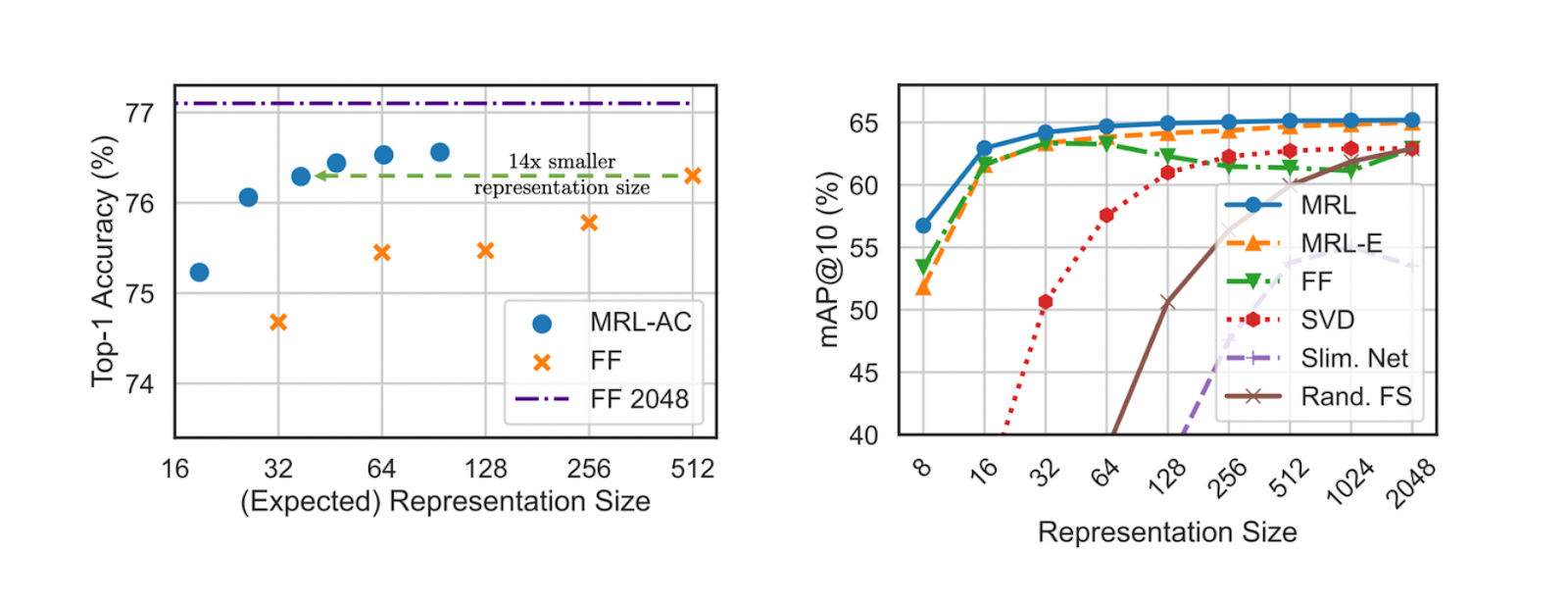 Figure- Top 1 accuracy of ResNet50 model in adaptive classification (left) and mAP of ResNet50 in image retrieval use case (right)
Figure: Top 1 accuracy of ResNet50 model in adaptive classification (left) and mAP of ResNet50 in image retrieval use case (right). Source.
Next, let’s discuss retrieval. As you might know, the goal of retrieval is to find a set of similar contexts for a given query. Therefore, the retrieval quality between ResNet50 trained with MRL and fixed-size feature representations using mean Average Precision (mAP) was tested. The MRL model shows an improvement in mAP of up to 3% compared to its fixed-size counterpart at every feature representation size, as illustrated in the visualization above.
Since we can utilize several feature representation sizes with MRL, it’s also particularly interesting to explore how we can speed up the retrieval process while maintaining accuracy with MRL. We can test it in a scenario called adaptive retrieval.
As mentioned earlier, there are two main stages in a retrieval process: shortlisting and reranking. The setup of adaptive retrieval involved using a 16-dimensional feature representation for shortlisting a set of 200 candidates, while a 2048-dimensional feature representation is used for reranking. This approach is compared with another method that uses a 2048-dimensional feature representation for both shortlisting and reranking.
On ImageNet-1K, using the MRL model can theoretically speed up the retrieval process by up to 128 times. We refer to this as theoretical because in real-world applications, we rarely use a naive nearest neighbor algorithm for retrieval tasks. Instead, approximate nearest neighbor (ANN) algorithms like FAISS, ANNOY, or HNSW are commonly implemented to enhance retrieval speed. In this case, the setup using the MRL model achieves a 14-fold speedup compared to retrieval processes using the HNSW algorithm on identical hardware.
A similar result was observed with the ImageNet-4K dataset, where the paper’s authors used an MRL model with a 64-dimensional feature representation for shortlisting and a 2048-dimensional representation for reranking. The results indicate a theoretical speedup of 32 times and a real-world speedup of six times.
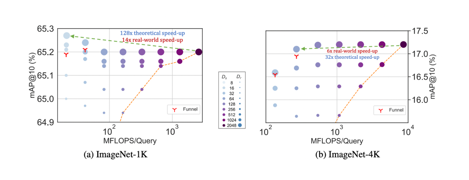 The trade-off between mAP@10 vs MFLOPs/Query for Adaptive Retrieval (AR) on ImageNet-1K (left) and ImageNet-4K (right).
The trade-off between mAP@10 vs MFLOPs/Query for Adaptive Retrieval (AR) on ImageNet-1K (left) and ImageNet-4K (right). Source.
MRL Approach Implementation
In this section, we’ll take a look at the simple implementation of the MRL approach. In particular, we’ll use an MPNet base model trained with the MRL approach on the NLI dataset to generate embeddings in different sizes. As you might already know, the original MPNet base model can only generate a 768-dimensional embedding. However, this trained MPNet model can generate embeddings in 768, 512, 256, 128, and 64 dimensions, where the weight of each dimension during training is set to 1.
We can use this model with the help of the SentenceTransformers library with the following code.
from sentence_transformers import SentenceTransformer

matryoshka_dim_short = 64
matryoshka_dim_long = 768
text = ["The weather is so nice!"]

short_embedding = SentenceTransformer("tomaarsen/mpnet-base-nli-matryoshka", truncate_dim=matryoshka_dim_short).encode(text)
long_embedding = SentenceTransformer("tomaarsen/mpnet-base-nli-matryoshka", truncate_dim=matryoshka_dim_long).encode(text)

print(f"Shape: {short_embedding.shape, long_embedding.shape}")
print(short_embedding[0][0:10])
print(long_embedding[0][0:10])
"""
Output:
Shape: ((1, 64), (1, 768))
[-0.33891088  0.01647538 -0.29915053  0.24952686 -0.04321517 -0.31616145
 -0.12996909 -0.05221268  0.02296597  0.07074839]
[-0.33891088  0.01647538 -0.29915053  0.24952686 -0.04321517 -0.31616145
 -0.12996909 -0.05221268  0.02296597  0.07074839]
 """
In the code above, we use the trained MPNet base model to generate embeddings in two different sizes: 64 and 768. Since the weight or scaling factor of each dimension is set to 1, then the two embeddings have identical elements, as you can see in the first 10 elements of two embeddings above.
Since the value of each element is identical, then the similarity between the two embeddings would be 1.
from sentence_transformers.util import cos_sim

similarities = cos_sim(short_embedding[0], long_embedding[0][:matryoshka_dim_short])
print(similarities)
# tensor([[1.]])
If you’d like to train your own model with the MRL approach, you can take a look at the official GitHub repo of this method.
Conclusion
The MRL approach introduces a solution to balance the cost-performance trade-off in machine learning. By enabling any machine learning model to produce feature representations of varying sizes, MRL provides the flexibility to optimize for either speed or accuracy depending on our use case and resources. We’ve seen that this adaptability is valuable in applications like classification and retrieval, where switching between smaller and larger representations can significantly enhance efficiency without sacrificing performance massively.
The experimental results demonstrate that MRL matches and often surpasses the accuracy of traditional fixed-size models across multiple domains, including text, vision, and multimodal tasks. Also, the approach's compatibility with existing architectures like ResNet50, ViT, and BERT highlights its applicability across different model modalities. With the potential for substantial speedups in real-world scenarios and improved retrieval quality, MRL represents a promising advancement for more efficient and versatile machine learning solutions.
Relate Resources
Keep Reading

Zilliz Cloud Delivers Better Performance and Lower Costs with Arm Neoverse-based AWS Graviton
Zilliz Cloud adopts Arm-based AWS Graviton3 CPUs to cut costs, speed up AI vector search, and power billion-scale RAG and semantic search workloads.

Announcing the General Availability of Zilliz Cloud BYOC on Google Cloud Platform
Zilliz Cloud BYOC on GCP offers enterprise vector search with full data sovereignty and seamless integration.
VidTok: Rethinking Video Processing with Compact Tokenization
VidTok tokenizes videos to reduce redundancy while preserving spatial and temporal details for efficient processing.
