Learn
Exploring Vector Database Use Cases

Powering Semantic Similarity Search in Computer Vision with State of the Art Embeddings

Jan 24, 202222 min read

Discover how to extract useful information from unstructured data sources in a scalable manner using embeddings.

Read the entire series

A whopping 90% of data created since the dawn of human civilization was produced in the past two years! The rate of data creation continues to increase with the proliferation of digital technologies such as social media and the internet of things (IoT) together with ever-faster wireless communication technologies such as 5G. However, most new data created is “Unstructured", such as text, images, audio, and video.

Unstructured data gets its name because it does not have an inherent structure, unlike a table of rows and columns. Instead, unstructured data contains information in one of several possible formats. For example, e-commerce images, customer reviews, social media posts, surveillance videos, speech commands, etc., are rich sources of information that do not follow the traditional tabular data format.

Recent advances in Artificial Intelligence (AI) and Machine Learning (ML) technologies have created a way to extract useful information from unstructured data sources in a scalable way by the use of “embeddings.” Converting unstructured data into embeddings and storing them on a vector database such as Milvus have enabled several excellent applications that were unimaginable just a few years back. Some example applications are visual image search, semantic text search, recommendation engines, fighting misinformation, drug discovery, etc.!

For this post, we’ll be using the Digikala Products Color Classification dataset from Kaggle to build a simple e-commerce image-based similar product search service. The dataset is licensed under GPL 2 license.

What is an embedding

Our computers cannot directly understand images or text the way we humans do. However, computers are good at understanding numbers! Thus, to help our computers understand the content of images or text, we need to convert them into a numeric representation. For example, if we consider the image use case, we are essentially “encoding” or “embedding” the context and scene of our image into a series of numbers in the form of a vector.

An “embedding” vector is a numeric representation of our image data so that our computers can understand the context and scene of our images.

Computers cannot understand images directly but, they can understand numbers very well!

Several libraries allow us to generate embeddings from our images. In general, we can group these libraries into two broad categories.

Libraries that provide ready-made APIs with pre-trained models: We probably do not need to train any models for many real-world problems involving images of everyday objects. Instead, we can rely on the many high-quality pre-trained models open-sourced by researchers worldwide. Researchers have trained these models to recognize and cluster several everyday objects from the ImageNet dataset.
Libraries that allow us to train and fine-tune our models: As the name suggests, for these models, we can bring our data and train models from scratch or fine-tune pre-trained models specifically for our use case. We will only need to go down this path if the pre-trained models don’t already provide good embeddings for our problem domain.

Let’s look at a few of the libraries for #1 in this post. But first, let’s load some image data to evaluate our embeddings in a similarity search application qualitatively.

Load Some Data

We first need to load some image data to test the various embedding strategies. For this post, let’s use the Digikala Products Color Classification dataset from Kaggle. The dataset contains images of more than 6K e-commerce products, perfect for testing an e-commerce image-based similar product search service.

Step 1: Setup a Kaggle Environment

Create an account on kaggle.com
Click on your profile picture and click on “Account” from the drop-down menu.
Scroll down to the “API” section.
Click on the “Create New API Token” button as shown in the image below to download a fresh token as a JSON file having a username and API key.
If you’re using macOS or Linux, copy the JSON file to the ~/.kaggle/ directory. On a Windows system, go to your root directory, then to the .kaggle folder, and copy the downloaded file to this folder. If the .kaggle directory doesn’t exist, please create it and copy the JSON file.

Create a new Kaggle API token.

Step 2: Download Data from Kaggle

We’ll be using Anaconda to manage a virtual environment for this project. You can install Anaconda from its website. Once you’ve downloaded and installed Anaconda, we can set up a new environment called semantic_similarity, install the necessary libraries such as kaggle and pandas, and download the entire dataset from kaggle.com by running the below commands in a terminal window. If you don’t want to use Anaconda, you can also use python’s venv to create and manage a virtual environment for this project.

# Create a directory for notebooks and another to download data 
mkdir -p semantic_similarity/notebooks semantic_similarity/data/cv 

# CD into the data directory
cd semantic_similarity/data/cv

# Create and activate a conda environment
conda create -n semantic_similarity python=3.8
conda activate semantic_similarity

## Create Virtual Environment using venv if not using conda
# python -m venv semantic_similarity
# source semantic_similarity/bin/activate

# Pip install the necessary libraries
pip install jupyterlab kaggle pandas matplotlib scikit-learn tqdm ipywidgets

# Download data using the kaggle API
kaggle datasets download -d masouduut94/digikala-color-classification

# Unzip the data into a fashion/ directory
unzip digikala-color-classification.zip -d ./fashion

# Delete the Zip file
rm digikala-color-classification.zip

The data contains over 6K images of various e-commerce products. We can see some sample images from the dataset in the image below. As you can notice, the dataset comprises various fashion products such as men’s attire, women’s attire, bags, jewelry, watches, etc.

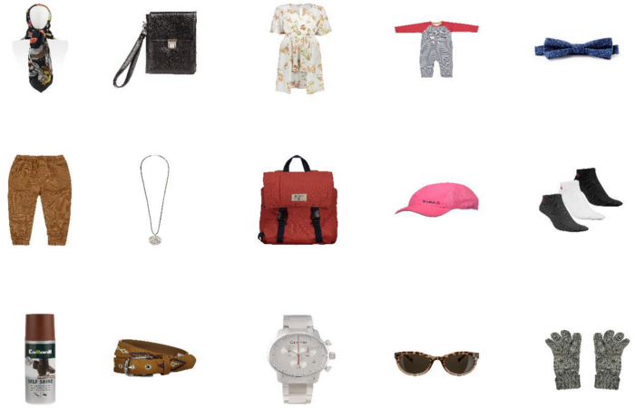Sample products available in the dataset. Composite image by Author using images from the Digikala Products Color Classification dataset.

Step 3: Move all the images from each folder to the parent folder

Let’s create a new jupyter notebook in the semantic_similarity/notebooks directory to test various embeddings strategies. First, let’s import the necessary libraries.

from matplotlib import pyplot as plt
import numpy as np
import os
import pandas as pd
from PIL import Image
from random import randint
import shutil
from sklearn.metrics.pairwise import cosine_similarity
import sys 
from tqdm import tqdm

tqdm.pandas()

The downloaded images are located in several sub-folders. Let’s move all of them into the main parent directory so that we can easily get all their paths.

def move_to_root_folder(root_path, cur_path):
    # Code from https://stackoverflow.com/questions/8428954/move-child-folder-contents-to-parent-folder-in-python
    for filename in os.listdir(cur_path):
        if os.path.isfile(os.path.join(cur_path, filename)):
            shutil.move(os.path.join(cur_path, filename), os.path.join(root_path, filename))
        elif os.path.isdir(os.path.join(cur_path, filename)):
            move_to_root_folder(root_path, os.path.join(cur_path, filename))
        else:
            sys.exit("Should never reach here.")

    # remove empty folders
    if cur_path != root_path:
        os.rmdir(cur_path)
        
move_to_root_folder(root_path='../data/cv/fashion', cur_path='../data/cv/fashion')

Code from StackOverflow, modified by Author.

Step 4: Load the image paths into a pandas dataframe

Next, let’s load the list of all the image file paths into a pandas dataframe.

# Path to all the downloaded images
img_path = '../data/cv/fashion'

# Find list of all files in the path
images = [
    f'../data/cv/fashion/{f}' 
    for f in os.listdir(img_path) 
    if os.path.isfile(os.path.join(img_path, f))
]

# Load the file names to a dataframe
image_df = pd.DataFrame(images, columns=['img_path'])
print(image_df.shape)
image_df.head()

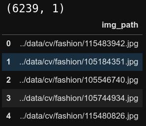First 5 rows in the dataframe.

Strategies for generating embeddings

Recent advances in Computer Vision technologies have opened up many ways to convert images into numeric embeddings. Let’s take a look at a few of them.

Flattening the raw pixel values
Convolutional neural networks pre-trained on classification objective
Convolutional neural networks pre-trained with Metric Learning objective
Image-Text Multimodal neural networks pre-trained with Metric Learning objective

Flattening the Raw Pixel Values

Color images consist of three-dimensional arrays of pixels. The 1st dimension is the height of the image, the 2nd dimension is the image’s width, and the final 3rd dimension is the color channels collectively known as RGB, which contains the Red, Green, and Blue, as shown in the figure below. The value of each pixel is an integer between 0 and 255, with 255 being the highest possible intensity.

Thus, the RGB value of (0,0,0) is an entirely dark or a pure black pixel, and (255,255,255) is a wholly saturated pure white pixel. All the other colors visible in our images are made up of various combinations of these fundamental three values of RGB. The RGB Color Codes Chart on the RapidTables website allows you to pick any color to view its RGB values, do try it out!

A color image consists of 3 channels, one for Red, one for Green, and one for Blue.

Given that images are a series of numbers in a 3D array format, converting them to a 1D vector using the reshape operation is trivial, as shown in the figure below. We can also normalize the pixels between 0 and 1 by dividing every pixel’s value by 255. We’ll do this in the code.

Flattening converts a 3D array to a 1D vector.

def flatten_pixels(img_path):
    # Load the image onto python
    img = Image.open(img_path).convert('RGB')
    
    # Reshape the image to 1D and normalize the values
    flattened_pixels = np.array(img).reshape(-1)/255.
    
    return flattened_pixels

# Apply the transformation to the dataframe
# Warning! Running only on a subset 1K rows of the data,
# Your computer might crash if you run on the entire dataset! 
# Better don’t run it. We have much better ways to generate embeddings!
pixels_df = styles_df.sample(1_000).reset_index(drop=True).copy()
pixels_df['flattened_pixels'] = pixels_df['img_path'].progress_apply(flatten_pixels)

Issues with this approach

Though this method is easy to understand and straightforward to implement, there are some severe drawbacks to this approach of “embedding” images into vectors.

Huge vectors: The images that we downloaded from Kaggle are pretty small in size [80 x 60 x 3] corresponding to the [Height x Width x Channels], and converting this 3D array to a 1D vector results in a vector of size 14400! That is a massive vector for such a small image! My computer crashed several times while generating this vector on our entire dataset. I ended up only running it on a smaller subset (1K rows) to illustrate this method.
Sparse vectors with a lot of empty (white) space: Visually inspecting the images in our fashion dataset, we notice large white areas in the picture. So, many elements of this 14400 element vector are just the value 255 (for white) and do not add any information related to the object in the image. In other words, this “embedding” scheme does not efficiently encode the object of the image but instead includes a lot of useless white space.
Lack of Local Structure: Finally, directly flattening an image loses all the local structure of the picture. For example, we identify the image of a human face by the relative positions of the eyes, ears, nose, and mouth. These are various “feature” level information that we would completely miss if we look at one row of pixels at a time. The impact of this loss is that an upside-down face would have a very different flattened embedding from a right side up face, even though both are pictures of the same human face!

We have mostly overcome these issues with the advent of novel neural network architectures based on the Convolutional Neural Network CNN and the Transformer architectures. The rest of this post dives into ways to use these neural networks to convert our images into embeddings.

Convolutional Neural Networks Pre-Trained on Classification Objective

Perhaps one of the most well-known computer vision tasks is classifying images into different categories. Generally, for this task, we would use a CNN model such as a ResNet as an encoder to convert the image into a vector and then pass this vector through a Multi-Layer Perceptron (MLP) model to determine the category of the image, as shown in the image below. Researchers would train this CNN + MLP model using Cross-Entropy loss to classify the image category accurately.

CNN.svg

This approach has provided state-of-the-art accuracies that even surpass the capabilities of most humans. After training such a model, we can leave out the MLP layer and directly take the output of the CNN encoder as an embedding vector for each input image.

In reality, we do not need to train our own CNN model from scratch for many real-world problems. Instead, we directly download and use models already trained to recognize everyday objects such as those categories in the ImageNet dataset. Towhee is a python library that quickly generates embeddings using these pre-trained models. Let’s take a look at how we can do so.

Towhee Pipelines

Towhee is a python library that provides extremely easy-to-use embedding generation pipelines. We can use towhee to convert an image to an embedding with less than five lines of code! First, let’s install towhee using pip in a terminal window.

# Activate the conda environment if not already done so
# conda activate semantic_similarity
pip install towhee

Next, in a Jupyter notebook cell, let’s import the library and instantiate a pipeline object.

from towhee import pipeline
embedding_pipeline = pipeline('image-embedding')

Next, let’s convert images to embeddings using the pipeline. This is just a single line of code! The output of the embedding pipeline has a few additional dimensions that we can strip away using np.squeeze.

styles_df['embedding'] = styles_df['img_path'].progress_apply(lambda x: np.squeeze(embedding_pipeline(x)))
styles_df.head()

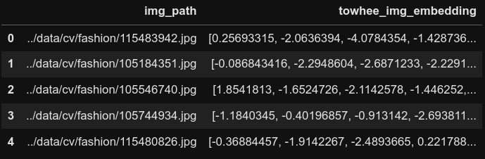First 5 rows of the dataframe post towhee embedding creation.

Before we proceed further, let’s create a helper function that takes in the column’s name that contains embeddings, an index of the data frame that serves as a query image, and the k number of similar images to search. The function calculates the cosine similarities between the embedding of the query image and the embeddings of all the other images in the dataframe to find the top k most similar images and displays them.

def plot_similar(df, embedding_col, query_index, k_neighbors=5):
    '''Helper function to take a dataframe index as input query and display the k nearest neighbors
    '''
    
    # Calculate pairwise cosine similarities between query and all rows
    similarities = cosine_similarity([df[embedding_col][query_index]], df[embedding_col].values.tolist())[0]
    
    # Find nearest neighbor indices
    k = k_neighbors+1
    nearest_indices = np.argpartition(similarities, -k)[-k:]
    nearest_indices = nearest_indices[nearest_indices != query_index]
    
    # Plot input image
    img = Image.open(df['img_path'][query_index]).convert('RGB')
    plt.imshow(img)
    plt.title('Query Product')
    
    # Plot nearest neighbors images
    fig = plt.figure(figsize=(20,4))
    plt.suptitle('Similar Products')
    for idx, neighbor in enumerate(nearest_indices):
        plt.subplot(1, len(nearest_indices), idx+1)
        img = Image.open(df['img_path'][neighbor]).convert('RGB')
        plt.imshow(img)
        plt.title(f'Cosine Sim: {similarities[neighbor]:.3f}')
    plt.tight_layout()

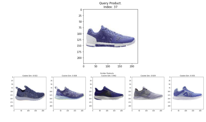
We can now test the quality of towhee’s embeddings by querying random images from the data frame and displaying the k most similar images using the above helper function. As shown below, the towhee embeddings are pretty spot-on for every query we run to find similar pictures from the entire set of images containing several different products like dresses, watches, bags, and makeup! It’s even more impressive considering we generated these embeddings with just three lines of code!

plot_similar(df=styles_df,
             embedding_col='embedding', 
             query_index=randint(0, len(styles_df)), # Query a random image
             k_neighbors=5)

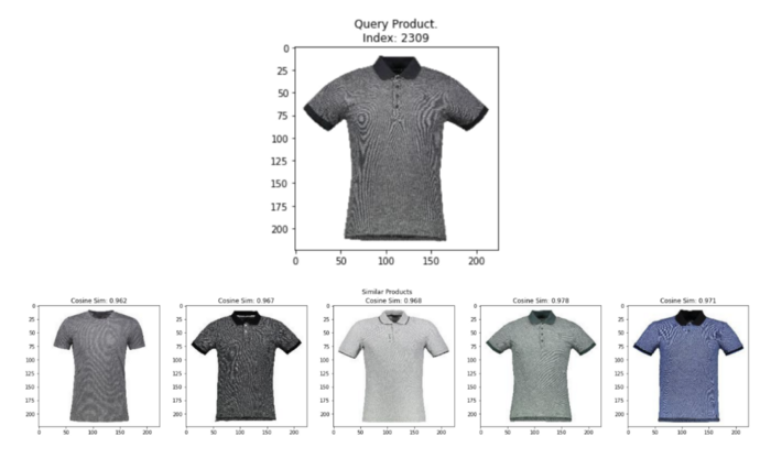Random query image and top 5 most similar images from towhee embeddings. Image by Author using images from the Digikala Products Color Classification dataset with GPL 2 license.

From the results, we can conclude that towhee is a great starting place for quickly generating embeddings for similarity search applications. However, we did not explicitly train these models to ensure similar images have embeddings identical to each other. Thus in the context of similarity search, the embeddings from such models may not be the most accurate for all use cases. The natural question you may be asking now is, “Is there a way to train models such that similar images have embeddings that are also similar to each other?” Thankfully, there is!

Convolutional Neural Networks Pre-Trained with Metric Learning Objective

Enter Metric learning, one of the most promising ways to generate embeddings, especially for similarity search applications. At its very fundamental level, in metric learning,

We use a neural network such as a CNN or a Transformer network to convert images to embeddings.
We construct these embeddings so that semantically similar images cluster nearer to each other while dissimilar images are further apart.

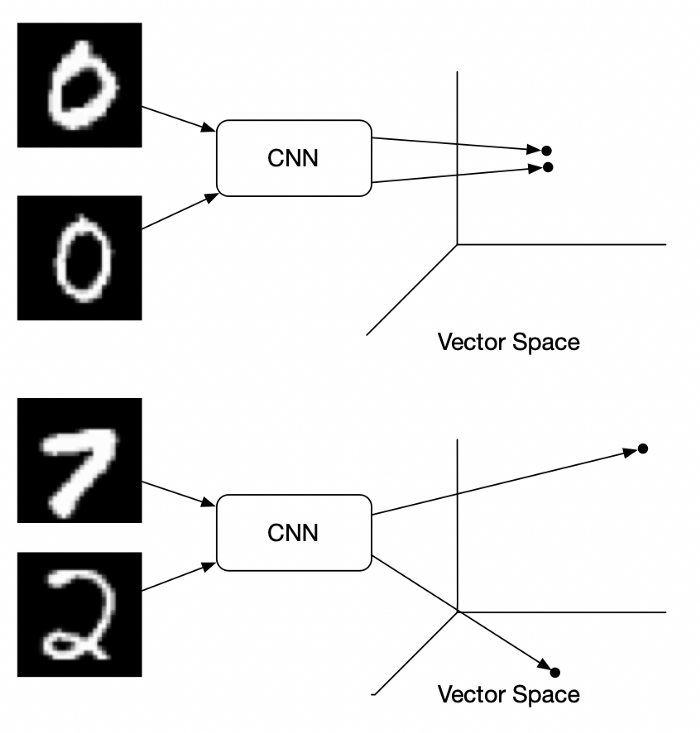Example of handwritten images in vector space. Image Source: Medium Blog Post by Brian Williams.

Training metric learning models requires innovation in the way the data is processed and how the model is trained.

1.Data: In metric learning, for each source image called “anchor” image, we require at least one similar image called “positive.” We can also incorporate a dissimilar third image, called “negative,” to improve the embedding representation. In recent approaches to metric learning for each source image, we synthetically generate an “anchor” and a “positive” image using various data augmentations, as shown in the image below. Since both images are variations of the same source image, labeling them as an anchor-positive pair is logical. On the other hand, we synthetically generate “negatives” by taking all the images other than the “anchor” in the same batch of images.

2.Model: Metric learning models mostly have a Siamese Network architecture. The anchor, positive and negative images are sequentially passed through the same model to generate embeddings that we then compare using special loss functions. One of such loss functions is called contrastive loss, where the model’s objective is to move the embeddings for the anchor and positive images closer together such that the distance between them is near 0. Conversely, the model aims to move the anchor and negative embeddings further away from each other such that the distance between them is large.

Anchor and Positive are both augmented Versions of the same source image. Image by Author using images from the Digikala Products Color Classification dataset with GPL 2 license. Inspired by the Google AI Blog.

After training the model with this approach, we can find the similarity between any two images by mathematically computing the distance between their embedding vectors using measures such as cosine distance. As shown in the image below, several distance measures exist, with cosine distance popular for comparing embeddings.

SimCLR is one of the popular approaches to generating image embedding using a type of metric learning called contrastive learning. Let’s look at SimCLR and how we can generate SimCLR embeddings on our dataset.

SimCLR: Simple Contrastive Learning

SimCLR stands for a Simple framework for Contrastive Learning of Visual Representations. In contrastive learning, the contrastive loss function compares whether two embeddings are similar (0) or dissimilar (1).

The great thing about SimCLR is that it’s a simple self-supervised algorithm (we do not need any labels for the image classes) that achieves performance on par with some Supervised approaches, as shown in the figure below!

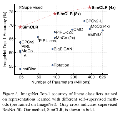Self-supervised SimCLR 4X achieves similar accuracy as a fully supervised ResNet50! Image source: SimCLR Paper.

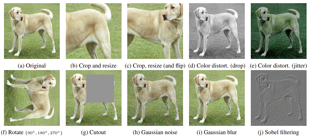Examples of possible image data augmentations. Image source: SimCLR Paper.

The fundamental idea of SimCLR is as follows.

1.Given an image, create two augmented versions of the same image. These augmentations can be cropping and resizing, color distortion, rotations, adding noise, etc. The below image shows some examples of augmentations.

2.The augmented versions of all images within a batch pass through a CNN encoder that converts the images to embeddings. These CNN embeddings then pass through a simple Multi-Layer Perceptron (MLP) with just one hidden layer to transform them into another space.

3.Finally, the embeddings at the output of the MLP are compared with each other using cosine distance. The model expects augmentations from the same image to have a cosine distance of 0, while augmentations from different images have a distance of 1. The loss function then updates the parameters of both the CNN and MLP such that the embeddings move closer to our expectations.

4.Once the training is complete, we don’t need the MLP anymore and directly use the output of the CNN encoder as our embeddings.

The below image explains the whole process conceptually. For more details, please take a look at this Google blog post.

SimCLR explained conceptually. Image by Author using images from the Digikala Products Color Classification dataset with GPL 2 license. Inspired by the Google AI Blog.

The authors ran several experiments and determined that random cropping and color distortion were the best combinations of augmentations, as shown below.

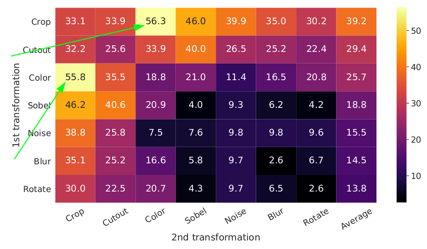Downstream model accuracy with different sets of data augmentations. Image source: SimCLR Paper.

Like Towhee, we use models pre-trained on ImageNet by other researchers directly to extract the SimCLR embeddings. However, as of this writing, to obtain the SimCLR pre-trained embeddings, we need to write several lines of code using the Pytorch Lightning Bolts library. I’ve adapted the below from the official Lightning Bolts documentation. First, install the necessary libraries using pip in a terminal window.

# Activate the conda environment if not already done so
# conda activate semantic_similarity
pip install lightning-bolts wandb gym opencv-python

Next, in a Jupyter notebook cell, let’s import the necessary libraries and set the device to cuda or cpu depending on whether your computer has a GPU.

from pl_bolts.models.self_supervised import SimCLR
import torch
from torch.utils.data import Dataset, DataLoader
from torchvision import io, transforms 

# Use GPU if it is available
device = torch.device('cuda' if torch.cuda.is_available() else 'cpu')

Next, let’s load the SimCLR model pre-trained on ImageNet and set it to eval mode because we only want to get embeddings out of the model and do not want to train it anymore.

# load resnet50 pre-trained using SimCLR on imagenet
weight_path = 'https://pl-bolts-weights.s3.us-east-2.amazonaws.com/simclr/bolts_simclr_imagenet/simclr_imagenet.ckpt'
simclr = SimCLR.load_from_checkpoint(weight_path, strict=False, batch_size=32)

# Send the SimCLR encoder to the device and set it to eval
simclr_resnet50 = simclr.encoder.to(device)
simclr_resnet50.eval();

The following two steps are specific to Pytorch; the underlying library used to implement the model. We first create a dataset that can take in our dataframe as input, read the images from the img_path column, apply some transformations, and finally create batches of images that we can feed into the model.

# Create a dataset for Pytorch
class FashionImageDataset(Dataset):
    def __init__(self, styles_df, transform=None):
        self.styles_df = styles_df
        self.transform = transform

    def __len__(self):
        return len(self.styles_df)

    def __getitem__(self, idx):
        # Load the Image
        img_path = self.styles_df.loc[idx, 'img_path']
        image = io.read_image(img_path, mode=io.image.ImageReadMode.RGB)/255.

        # Apply Transformations
        if self.transform:
            image = self.transform(image)
            
        return image

# Transforms
## Normalize transform to ensure the images have similar intensity distributions as ImageNet
## Resize transform to ensure all images in a batch have the same size 
transformations = transforms.Compose([
    transforms.Normalize((0.485, 0.456, 0.406), (0.229, 0.224, 0.225)),
    transforms.Resize(size=(64, 64))
])
    
# Create the DataLoader to load images in batches
emb_dataset = FashionImageDataset(styles_df=styles_df, transform=transformations)
emb_dataloader = DataLoader(emb_dataset, batch_size=32)

Finally, we can iterate over the batches in the dataloader, generate the embeddings for all the images and store it back as a column in our dataframe.

# Create embeddings
embeddings = []
for batch in tqdm(emb_dataloader):
    batch = batch.to(device)
    embeddings += simclr_resnet50(batch)[0].tolist()

# Assign embeddings to a column in the dataframe
styles_df['simclr_embeddings'] = embeddings
styles_df.head(2)

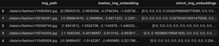First 5 rows of the dataframe post SimCLR embedding generation.

Now comes the fun part! We can test the quality of the SimCLR embeddings with the same helper function. We query random images from the data frame and display the k most similar images. As shown below, the SimCLR embeddings are also quite spot on to find similar images for every query we run!

plot_similar(df=image_df,
             embedding_col='simclr_img_embeddings', 
             query_index=randint(0, len(image_df)), 
             k_neighbors=5)

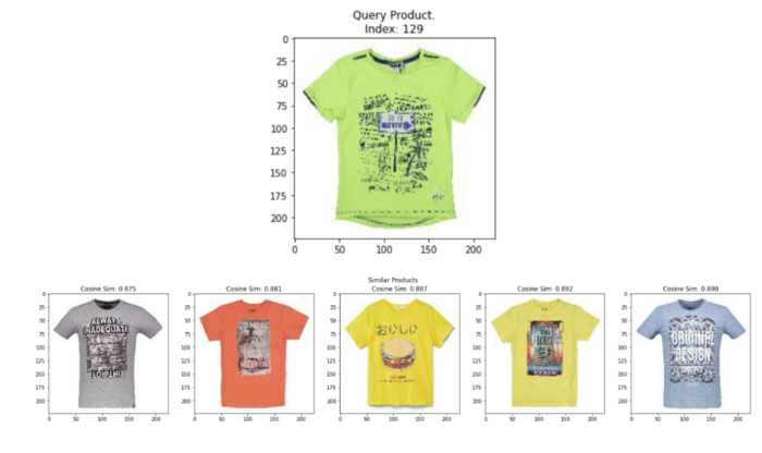Random query image and top 5 most similar images from SimCLR embeddings. Image by Author using images from the Digikala Products Color Classification dataset with GPL 2 license.

Image-Text Multimodal Neural Networks Pre-Trained with Metric Learning Objective

Finally, there have been tremendous improvements in models that embed both images and text into a unified embedding space Open AI’s CLIP Paper, Google’s ALIGN Paper, Microsoft’s PixelBERT Paper which opens up several excellent applications such as Image-To-Text and Text-To-Image similarity search. Currently, one of the most popular models in this paradigm is CLIP (Contrastive Language-Image Pre-Training).

CLIP is a neural network that builds upon the metric learning framework. Instead of training on purely image anchor-positive pairs, CLIP uses an image as the anchor and the corresponding text description as the positive to construct image-text pairs. We can use CLIP in several applications, including Text-to-Image, Image-To-Text, Image-to-Image, and Text-to-Text similarity search.

The images are passed through a ResNet or a ViT encoder to generate the image embeddings. The text descriptions are fed through a GPT based encoder to generate text embeddings. CLIP jointly trains both the image and text encoders such that within a batch of $N$ image-text pairs, the embedding of the $i^{th}$ image has the highest dot product with the embedding of the $i^{th}$ text as shown in the figure below.

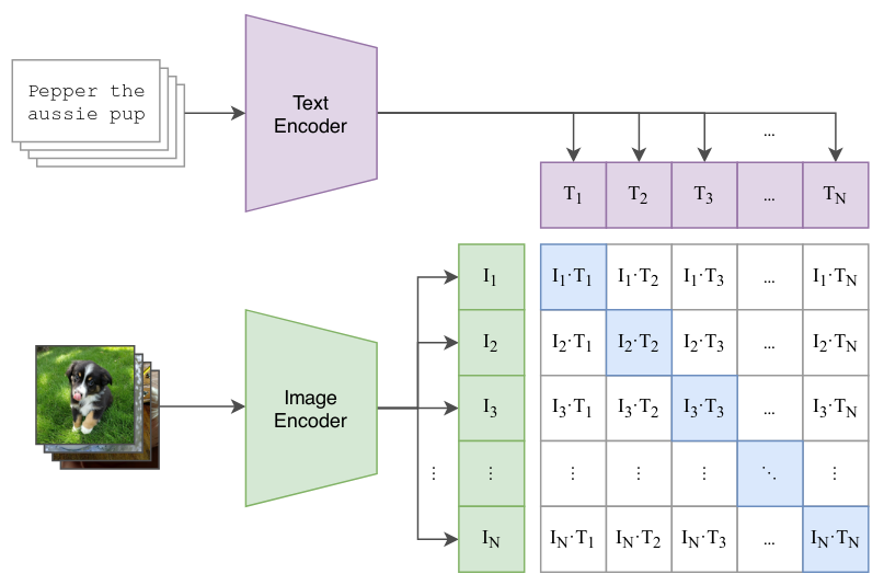CLIP’s Contrastive pre-training. Image Source: CLIP Paper

After the training is complete, we can find the row of text most similar to a query image by simply converting both into their respective embeddings and comparing them using dot product or cosine distance, as shown in the image below. Conversely, we can also search for most similar images given a query text in the same way. Let’s see how we can implement this on our example problem.

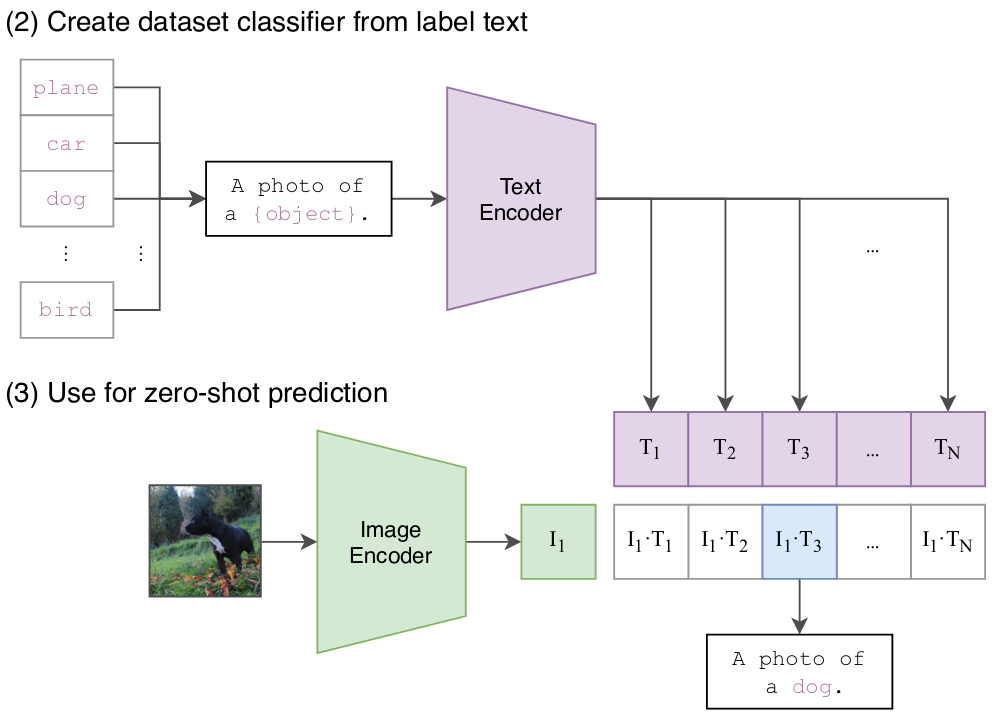CLIP 2.png

Sentence Transformers (CLIP)

Generating CLIP embeddings on our data is straightforward with the excellent Sentence-Transformers library. However, due to OS limitations on the number of files we can open at a time, we need to write a few lines of boilerplate code when working with tens of thousands of images. First, install the necessary libraries using pip in a terminal window.

# Activate the conda environment if not already done so
# conda activate semantic_similarity
pip install sentence_transformers spacy ftfy

Next, in a Jupyter notebook cell, let’s import the library and instantiate a CLIP model.

from sentence_transformers import SentenceTransformer
model = SentenceTransformer('clip-ViT-B-32')

Next, we need to iterate over 10K images at a time to get around an OS limitation on the number of files that can be open at a time. We load all the images during each iteration and generate CLIP embeddings.

# Initialize an empty list to collect embeddings
clip_embeddings = []

# Generate embeddings for 10_000 images on each iteration
step = 10_000

for idx in range(0, len(styles_df), step):
    # Load the `step` number of images
    images = [
        Image.open(img_path).convert('RGB') 
        for img_path in styles_df['img_path'].iloc[idx:idx+step]
    ]
    
    # Generate CLIP embeddings for the loaded images
    clip_embeddings.extend(model.encode(images, show_progress_bar=True).tolist())

# Assign the embeddings back to the dataframe
styles_df['clip_image_embedding'] = clip_embeddings

styles_df.head()

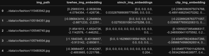First 5 rows of the dataframe post CLIP image embedding generation.

Now that we have the CLIP embeddings for all our images, we can use the same helper function to test the quality of the embeddings. We query random images from the data frame and display the k most similar images. As shown below, the CLIP embeddings are also quite spot on to find similar images for every query we run!

plot_similar(df=styles_df,
             embedding_col='clip_image_embedding', 
             query_index=randint(0, len(styles_df)), 
             k_neighbors=5)

Random query image and top 5 most similar images from CLIP image embeddings. Image by Author using images from the Digikala Products Color Classification dataset with GPL 2 license.

Though we had to write some additional code to generate the CLIP embeddings, one significant advantage it provides is Text to Image search. In other words, we can search for all the images that match a given text description. Let’s take a look at this below.

Since we’ve already converted the images to CLIP embeddings, we now only need to convert the text query to CLIP embedding. Then we can search for similar products by using cosine similarity between the text embedding and all the image embeddings in the dataframe. We’ll write a simple helper function to do all this for us, as shown below. Finally, we’ll plot all the similar k product images.

def text_image_search(text_query, df, img_emb_col, k=5):
    '''Helper function to take a text query as input and display the k nearest neighbor images
    '''
    
    # Calculate the text embeddings
    text_emb = model.encode(text_query).tolist()
    
    # Calculate the pairwise cosine similarities between text query and images from all rows
    similarities = cosine_similarity([text_emb], df[img_emb_col].values.tolist())[0]
    
    # Find nearest neighbors
    nearest_indices = np.argpartition(similarities, -k)[-k:]
    
    # Print Query Text
    print(f'Query Text: {text_query}')
    
    # Plot nearest neighbors images
    fig = plt.figure(figsize=(20,4))
    plt.suptitle('Similar Products')
    for idx, neighbor in enumerate(nearest_indices):
        plt.subplot(1, len(nearest_indices), idx+1)
        img = Image.open(df['img_path'][neighbor]).convert('RGB')
        plt.imshow(img)
        plt.title(f'{df["productDisplayName"][neighbor]}\nCosine Sim: {similarities[neighbor]:.3f}')
    plt.tight_layout()

Semantic Similarity Search in Computer Vision

Now we can use our helper function to test out sample text queries. As shown in the image below, if our test query is "a photo of a women’s dress," the most similar products are all dresses for women! Even though each product’s title doesn’t explicitly specify the word “dress,” the CLIP model was able to infer these images are most related to the query “women’s dress” just from the text and image embeddings. Go ahead and try it out with other queries!

text_query = "a photo of a women's dress"
text_image_search(text_query, 
                  df=styles_df, 
                  img_emb_col='clip_image_embedding', 
                  k=5)

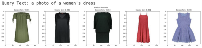Random query image and top 5 most similar images from CLIP text embeddings. Image by Author using images from the Digikala Products Color Classification dataset with GPL 2 license.

Conclusion

The current state of the art in Deep Learning research and Open Source code libraries have opened up many easy ways to generate high-quality embeddings from image and text data. These off-the-shelf embeddings are an excellent starting point for building a prototype for many real-world problems! The below flowchart can help to choose initial embeddings to use. However, constantly evaluate the accuracy of the embedding model on some complex sample queries before deploying any single one to production!

Talking about production, the dataset we used here was a toy dataset of only 44K images. In real-world applications, such as an e-commerce store, you would have hundreds of millions of product images to embed, store and perform nearest neighbors search within a fraction of a second! The scale of the problem requires using a powerful Vector Search database such as Milvus! You can learn more about vector databases at this Link.

Please visit our “learn” channel for more inspiration on the various cool applications of embeddings and vector similarity databases!

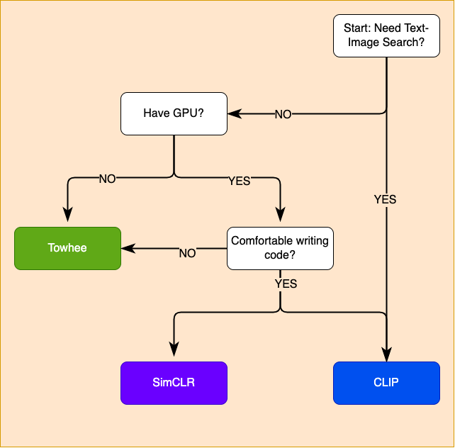Choosing an embedding approach. Image by Author

Updated on Mar 28, 2025

Marie Stephen Leo

Next: Supercharged Semantic Similarity Search in Production

Content

Start Free, Scale Easily

Try the fully-managed vector database built for your GenAI applications.

Try Zilliz Cloud for Free

Share this article

Keep Reading

Image-based Trademark Similarity Search System: A Smarter Solution to IP Protection

Learn how to use a vector database to build your own trademark image similarity search system that could save you from intellectual property lawsuits.

Proximity Graph-based Approximate Nearest Neighbor Search

Learn what PG-based ANNS is and how to optimize the algorithm to achieve a trade-off between search accuracy and efficiency.

How to Best Fit Filtering into Vector Similarity Search?

Learn about three types of attribute filtering in vector similarity search and explore our optimized solution to improve the efficiency of similarity search.