Blog
From CLIP to JinaCLIP: General Text-Image Representation Learning for Search and Multimodal RAG

From CLIP to JinaCLIP: General Text-Image Representation Learning for Search and Multimodal RAG

Oct 01, 202416 min read

Recently, the surge of multimodal embedding models has captured attention across various industries, transforming how machines interpret text and images. However, despite significant strides, these models face core challenges, one of which is the modality gap. This gap presents itself in how image and text embeddings are spatially distant in the latent space, even when describing the same object.

At a recent Unstructured Data Meetup hosted by Zilliz, Bo Wang, Engineering Manager at Jina AI, took us through the complexities of the modality gap and the transition from OpenAI’s CLIP model to JinaCLIP.

In this blog, we will recap his main points and also implement a multimodal similarity search system. This system will use JinaCLIP to generate multimodal embeddings and the Milvus vector database to store and retrieve similar embeddings given a certain query. For more details, we recommend you watch Bo’s full take on YouTube.

What Makes a Good Embedding Model?

An embedding model’s primary function is to map things like texts and images into vectors, numerical representations that capture semantic relationships within the data. For instance, the distance between two vectors should reflect the similarity of the two items they represent, be it two images, two texts, or one of each.

Embedding models are at the core of modern AI tasks like semantic search, image retrieval, and more. But what makes an embedding model good?

Versatility Across Domains

A good embedding model should perform well across a wide range of domains without requiring fine-tuning. This adaptability ensures the embeddings are universally useful, whether the input is text, images, or other data types. For instance, if an image is embedded into a vector space and a related text is embedded in the same space, the two embeddings should be close together, signifying their semantic similarity. This broad applicability is essential for AI tasks like similarity search, image retrieval, and cross-domain applications.

Accurate Semantic Similarity

A key characteristic of a good embedding model is its ability to connect left and right by producing embeddings with high similarity scores for semantically related items. This goes beyond just text data, it applies to any multimodal inputs. Whether comparing text to text, image to image, or text to image, the model should reflect the correct relationships through the proximity of the embeddings in vector space.

However, older models that connected text and image modalities had a harder time achieving this goal. They relied on manual processes, such as tagging images or using surrounding text, to establish connections. These methods resulted in poor generalization, particularly in out-of-distribution scenarios.

The Challenge of Multimodal Tasks

Before the introduction of models like CLIP, connecting modalities (text and images) was a highly manual and hypothesis-driven task. Whether it was Flickr tags or textual descriptions added by users, the process was far from seamless. Supervised approaches, often using classifier labels, were prone to instability, and their out-of-domain performance was unsatisfactory. This meant that while you could connect images and texts, the results weren’t always consistent, especially when the input was complex.

To solve this problem, CLIP, a contrastive language-image pretraining model, was developed to improve the performance of multimodal models by training them on image-text pairs. CLIP's ability to align the two modalities in a shared embedding space was innovative. However, this model also has its limitations.

CLIP Model: A Breakthrough With Restrictions

CLIP set a new standard by training two separate encoders, one for text and one for images. The core idea was to learn a shared embedding space where text and image vectors could coexist, with semantically similar texts and images sitting closer together. The results were impressive: CLIP allowed for multimodal tasks using a simple cosine similarity function.

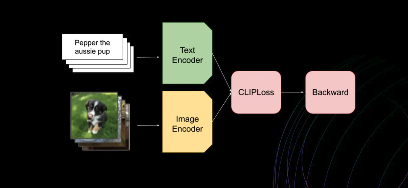Figure: How the CLIP model works

However, CLIP has its shortcomings. One significant issue is its inability to handle text-only tasks effectively. Since CLIP was primarily optimized for short captions (often fewer than 77 characters), longer texts pose a challenge. Furthermore, CLIP lacked hard-negative examples in its training process. Hard negatives are examples that are close but incorrect and are crucial for refining models, especially in tasks like text retrieval. Without them, CLIP’s performance plateaued on tasks requiring detailed text understanding.

Transitioning to JinaCLIP: Addressing Clip’s Shortcomings

JinaCLIP builds upon the original CLIP architecture to address its limitations. It expands the text input and uses an adapted BERT v2 architecture for text encoding. For image processing, JinaCLIP incorporates the EVA-02 model. The training process of JinaCLIP, focuses on overcoming the challenges posed by short text inputs in image captions and introducing hard negatives. This process occurs in three stages as shown below:

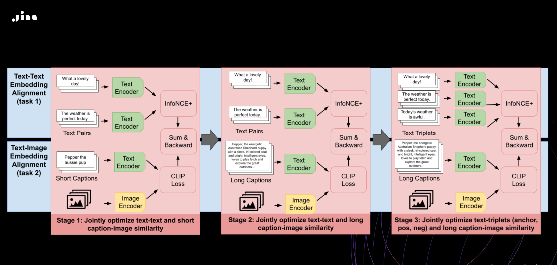Figure: Training Process of JinaCLIP

The stages are alignment learning, long-text integration, and fine-tuning:

Alignment Learning with Short Texts and Captions: In this stage, the model is trained using both captioned image data and text pairs with similar meanings. The objective is to align image and text embeddings by jointly optimizing for text-image and text-text similarity. This co-training process ensures that while the model learns to associate text with images, it also maintains its text-only capabilities. Though the text-only performance slightly declines compared to training exclusively on text pairs, this phase preserves a balanced approach.
Integration of Long Text Descriptions: During the second stage, synthetic data is introduced to train the model. This data aligns images with longer texts generated by AI models, describing the content in greater detail. Concurrently, text-only pairs continue to be used for training. The model learns to handle more extensive text descriptions while maintaining alignment with the images, enhancing its ability to understand both short and long text-image relationships.
Fine-Tuning with Text Triplets and Hard Negatives: The final stage focuses on using text triplets that include hard negatives, pairs of texts where two are semantically similar, but one is deliberately different. This helps the model make finer semantic distinctions, especially in text-only scenarios. At the same time, the model continues to train with synthetic image-long text pairs. This phase significantly improves the model's text-only performance, all while ensuring that the image-text alignment learned in earlier stages remains robust.

This approach maintains strong performance in multimodal tasks while enhancing capabilities in text-only scenarios. Let's see how this new approach compares to the original Clip.

Performance metrics indicate changes in retrieval performance compared to the original CLIP model: a 165% change in text-to-text, 12% in image-to-image, 6% in image-to-text, and 2% in text-to-image retrieval as shown in the image below.

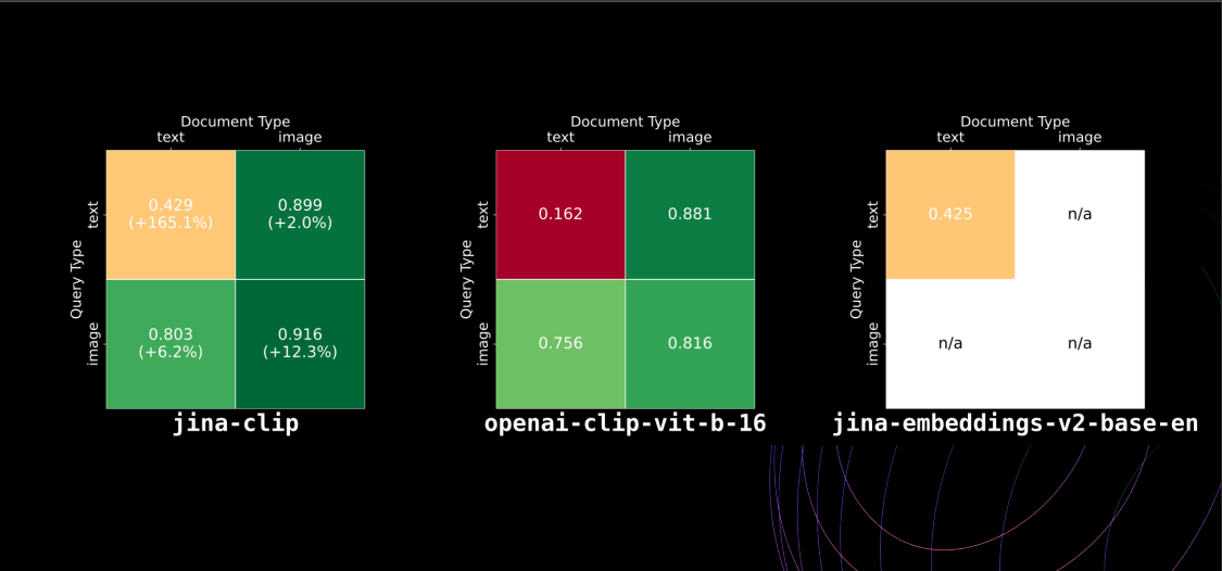Figure: Model performance comparison between jina-clip, openai-clip-vit-b-16, and jina-embeddings-v2-base-en

The new training process enhances generalization across tasks and helps reduce the modality gap. Let’s discuss the modality gap, a major obstacle in multimodal AI models, and why this problem happens.

The Modality Gap: Why It Happens

The modality gap is the spatial separation between embeddings from different input types, such as texts and images that are semantically similar but far apart in the vector space. This gap weakens the effectiveness of multimodal retrieval systems, as the embeddings don’t fully reflect the true relationship between related inputs. As you can see in the image below, the representation looks like a truncated cone, with image embeddings at one end and text embeddings at the other clearly showing the modality gap.

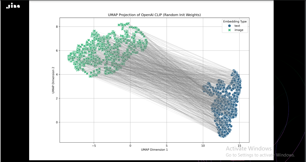Figure: The initial positions of image and text embeddings in Jina CLIP, with entirely randomized weights and no prior training, projected into two dimensions

There are a few key reasons why this gap arises, even in modern models:

The Cone Effect During Initialization

Multimodal models, particularly those that handle text and image inputs, often use separate encoders for each modality. These encoders are typically initialized with random or pre-trained weights, which causes text embeddings to cluster in one region of the vector space and image embeddings in another, as seen in the above image. This initial separation, called the cone effect, makes it difficult for embeddings from different modalities (e.g., images and related texts) to align properly. For instance, the text embedding for a fluffy cat and the image embedding of a cat may start far apart due to this initialization bias, even though they are semantically related.

Temperature Scaling

During training, AI models use a technique called temperature scaling in their contrastive loss function to adjust how closely embeddings are aligned. While it helps fine-tune the distances between embeddings, temperature scaling can also inadvertently preserve the initial separation between modalities, reinforcing the modality gap. For example, if temperature scaling isn’t carefully tuned, the embeddings for a playful puppy and the image of a dog might remain too far apart in the vector space, even though they describe the same concept.

In-Batch False Negatives

When training with large datasets, non-matching pairs of data points (e.g., an image of a dog paired with the text “a red apple”) are treated as negative examples. However, these false negatives might still share some semantic overlap. For instance, if both items relate to a broad category of animals (e.g., a picture of a dog and the text “a playful wolf”), the model could push these embeddings farther apart than necessary, further worsening the modality gap by incorrectly treating them as fully unrelated.

Understanding why the modality gap happens is only the first step. To bridge this gap, various training strategies have been developed to bring embeddings from different modalities closer together, ensuring more accurate retrieval in multimodal tasks.

Addressing the Modality Gap: Training Techniques and Beyond

The modality gap is a structural issue that doesn’t have an easy solution, but there are strategies to mitigate its impact. The key is to reduce the separation between embeddings from different modalities during training, ensuring that images and texts that belong together are mapped closer in the vector space.

Higher Temperature Scaling

In practice, increasing the temperature during training can encourage embeddings from different modalities to move closer together by adding more randomness to the model’s learning process. For example, increasing temperature can help align the embeddings of an image of a cat and the text “a fluffy cat” more closely. However, this comes at the cost of slower convergence and requires more computational resources. While models trained with high-temperature scaling tend to improve the alignment of text and image embeddings, the trade-off is often longer training times and greater computational demands.

Hard-Negative Sampling

Introducing hard-negative examples, non-matching pairs that are semantically close is another technique for reducing the modality gap. These hard-negative pairs push the model to learn finer distinctions between related concepts, improving retrieval accuracy. For instance, pairing an image of a cat with the text “a small tiger” might seem like a mismatch, but the model learns that these two inputs have overlapping semantics (both are felines) and should still be somewhat aligned in the embedding space. This process teaches the model to recognize both the similarities and differences between related concepts, refining its ability to differentiate between near matches.

Multimodal Retrieval with Milvus and JinaCLIP: A Practical Example

Now that we’ve explored the technical reasons behind the modality gap, let’s dive into a practical example of how to build a multimodal retrieval system using Milvus, an open-source vector database, and JinaCLIP.

Milvus manages, searches, and queries high-dimensional vectors, making it an ideal solution for multimodal retrieval tasks and Retrieval Augmented Generation (RAG) tasks. Whether you’re dealing with text, images, or other data types, Milvus enables you to store embeddings efficiently and retrieve relevant results using advanced similarity search techniques.

In this section, we’ll walk through the process of using Milvus to create a multimodal retrieval system that handles text and image embeddings. The system will allow users to input either text or images and retrieve the most semantically relevant results from a mixed dataset.

Step 1: Setting Up the Environment

First, we need to install the libraries we will need for our system in our environment:


!pip install pymilvus transformers torch timm

Then, we need to import the necessary libraries and set up our encoder class.


# Import necessary libraries

from transformers import AutoModel

from pymilvus import MilvusClient

import torch

# Define Encoder class to handle text and image embedding generation

class Encoder:

    def __init__(self, model_name: str):

        # Initialize the model (AutoModel from transformers instead of SentenceTransformer)

        self.model = AutoModel.from_pretrained(model_name, trust_remote_code=True)

    def encode_text(self, text: list[str]) -> list[float]:

        # Generate embeddings for text only

        with torch.no_grad():

            text_emb = self.model.encode_text(text)

        return text_emb

    def encode_image(self, image_urls: list[str]) -> list[list[float]]:

        # Generate embeddings for images only

        with torch.no_grad():

            image_emb = self.model.encode_image(image_urls)

        return image_emb

# Initialize the encoder with the model jinaai/jina-clip-v1

model_name = "jinaai/jina-clip-v1"

encoder = Encoder(model_name)

In the above code, we first import the required libraries: AutoModel from transformers for our encoding model, MilvusClient for interacting with Milvus, and torch for tensor operations.

We then define an Encoder class that wraps the AutoModel from transformers. The encode_text and encode_image methods use the model to generate embeddings for text and images, respectively. The torch.no_grad() context manager is used to disable gradient calculation, which isn't needed for inference and saves memory.

We finally initialize the encoder with the jinaai/jina-clip-v1 model, which can encode both text and images into a shared embedding space.

Step 2: Preparing the Data

Next, we'll prepare our sample data for embedding and insertion into Milvus.


# Load data: images and text for embeddings

sentences = ['A blue cat', 'A red cat', 'A red cat generated by AI', 'A dog biting on a stick']

image_urls = [

    'https://i.pinimg.com/600x315/21/48/7e/21487e8e0970dd366dafaed6ab25d8d8.jpg',

    'https://i.pinimg.com/736x/c9/f2/3e/c9f23e212529f13f19bad5602d84b78b.jpg',

    'https://images.fineartamerica.com/images/artworkimages/mediumlarge/1/red-cat-art-3771-bb-james-ahn.jpg',

    'https://images.squarespace-cdn.com/content/v1/54822a56e4b0b30bd821480c/29708160-9b39-42d0-a5ed-4f8b9c85a267/labrador+retriever+dans+pet+care.jpeg?format=1500w'

]

# Generate embeddings for text and images

text_embeddings = encoder.encode_text(sentences)

image_embeddings = encoder.encode_image(image_urls)

# Ensure consistent dimensions

dim = len(image_embeddings[0])

Here, we define lists of sample sentences and image URLs. The URLs contain images of red cats, blue cats, and a dog. We then use our encoder to generate embeddings for both the text and images. The dim variable stores the dimension of the embeddings, which we'll need when creating our Milvus collection.

Step 3: Setting Up Milvus

Now, we'll set up our Milvus client and create a collection for our multimodal data.


# Insert embeddings into Milvus

collection_name = "multimodal_rag_demo"

milvus_client = MilvusClient(uri="./milvus_demo.db")

# Check if collection exists and drop it if so

if milvus_client.has_collection(collection_name):

    print(f"Collection {collection_name} already exists. Deleting it...")

    milvus_client.drop_collection(collection_name)

# Create Milvus collection

milvus_client.create_collection(

    collection_name=collection_name,

    auto_id=True,

    dimension=dim,

    enable_dynamic_field=True,

)

We initialize a Milvus client and connect to a local database file. We check if a collection with our desired name already exists and, if so, drop it to ensure a clean slate.

We then create a new collection with the specified name. The auto_id=True parameter tells Milvus to automatically generate IDs for our entries. We set the dimension to match our embeddings and enable dynamic fields, which allows us to add additional metadata to our entries.

Step 4: Creating an Index

Before inserting data, we'll create an index to optimize search performance:


index_params = MilvusClient.prepare_index_params()

index_params.add_index(

    field_name="vector",  # The field to be indexed (your embedding field)

    metric_type="COSINE",  # Can be L2, COSINE, etc.

    index_type="FLAT",  # FLAT ensures exact search, ideal for small datasets

)

# Create the index for the collection

milvus_client.create_index(collection_name, index_params)

print(f"Index created successfully for collection: {collection_name}")

The above code creates a FLAT index using cosine similarity as the distance metric.

Step 5: Inserting Data into Milvus

With our collection and index set up, we can now insert our data into Milvus.


data_to_insert = []

# Insert text embeddings

for idx, txt_emb in enumerate(text_embeddings):

    data_to_insert.append({"text": sentences[idx], "vector": txt_emb})

# Insert image embeddings

for idx, img_emb in enumerate(image_embeddings):

    data_to_insert.append({"image_url": image_urls[idx], "vector": img_emb})

# Insert data into Milvus

insert_result = milvus_client.insert(

    collection_name=collection_name,

    data=data_to_insert,

)

print(f"Insert result: {insert_result}")

milvus_client.load_collection(collection_name)

In the above code, we create a list of dictionaries, each containing either a text sentence or an image URL, along with its corresponding embedding vector. We then use the Milvus client's insert method to add this data to our collection. After insertion, we load the collection into memory to prepare for searching.

Step 6: Performing Multimodal Search

Finally, we perform a multimodal search using both image and text queries.


# Multimodal search with a combination of image and text query

query_image_url = 'https://imgcdn.stablediffusionweb.com/2024/4/5/5e70d71c-a7f6-44e9-972d-8c5a27d45c3d.jpg'

query_text = "Give me similar red cats"

# Generate query embedding (image + text)

query_embedding_image = encoder.encode_image([query_image_url])[0]

query_embedding_text = encoder.encode_text([query_text])[0]

# Perform search in Milvus using image embedding

search_results_image = milvus_client.search(

    collection_name=collection_name,

    data=[query_embedding_image],

    output_fields=["image_url", "text"],  # Ensure both fields are included in the results

    limit=5,  # Number of results to return

    search_params={"metric_type": "COSINE", "params": {"nprobe": 10}}

)

# Perform search in Milvus using text embedding

search_results_text = milvus_client.search(

    collection_name=collection_name,

    data=[query_embedding_text],

    output_fields=["image_url", "text"],  # Ensure both fields are included in the results

    limit=5,  # Number of results to return

    search_params={"metric_type": "COSINE", "params": {"nprobe": 10}}

)

# Retrieve and print results from image query

print("Image Query Results:")

for result in search_results_image:

    for hit in result:

        image_url = hit['entity'].get('image_url')

        text = hit['entity'].get('text')

        if image_url:

            print(f"Retrieved Image URL (from image query): {image_url}")

        if text:

            print(f"Retrieved Text (from image query): {text}")

# Retrieve and print results from text query

print("Text Query Results:")

for result in search_results_text:

    for hit in result:

        image_url = hit['entity'].get('image_url')

        text = hit['entity'].get('text')

        if image_url:

            print(f"Retrieved Image URL (from text query): {image_url}")

        if text:

            print(f"Retrieved Text (from text query): {text}")

In the above code, we demonstrate the process of performing a multimodal search. We begin by defining both a query image URL and a query text. The query image looks like this:

Figure 2: Query input image of a red and white cat

Source

We then encode these queries using our encoder to generate their respective embeddings. We then conduct two separate searches in Milvus: one using the image embedding and another using the text embedding. For each search, we request both the image_url and text fields in the output, enabling us to retrieve both types of data. We limit our results to 5 for each search and employ cosine similarity as our distance metric. The nprobe parameter in our search parameters allows us to fine-tune the number of clusters to search, offering a balance between search speed and accuracy. Lastly, we display the results, showcasing which images or texts were retrieved for each query type, thus demonstrating the system's ability to handle and correlate both text and image-based queries.

You can find the full code here.

Here are sample results:

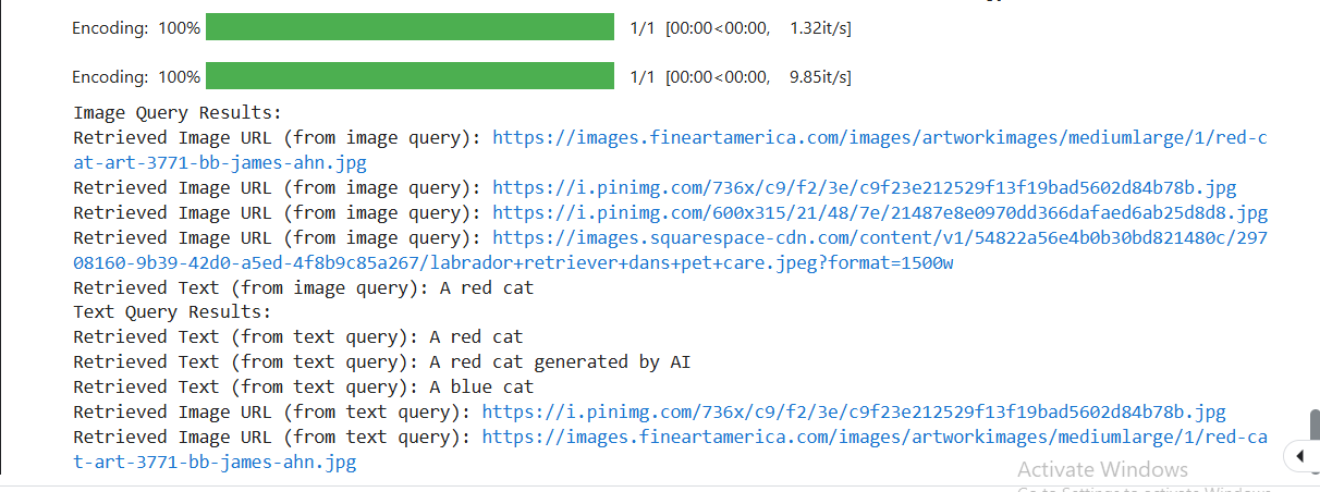
As you can see when we use an image to conduct a vector search we get both image URLs and text related to the image and vice versa. This is the power of Multimodal search. Here is one of the images that is retrieved as a similar image in both cases.

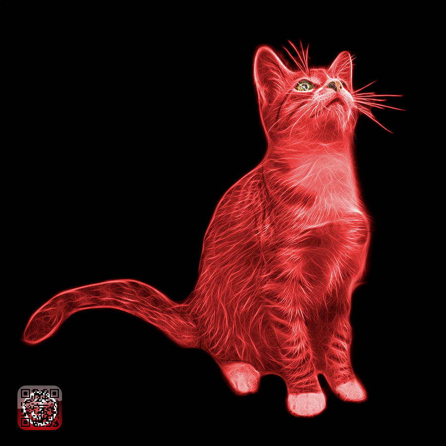Figure 3: Output image of a red cat after conducting a similarity search in Milvus

As you can see, the image is similar to the red cat image we gave the system as our query.

You can add a reranker to this system to arrange the search results in terms of relevance, with the top relevant results coming on top. Although, as it is evident, Milvus does a good job of retrieving the best matches first. You can also advance this system to create a multimodal RAG system.

Conclusion

Bo Wang explained the intricacies of bridging the modality gap in multimodal models and showcasing the transition from CLIP to JinaCLIP. He broke down the key challenges of text-image alignment and demonstrated how JinaCLIP addresses these issues.

In this article, we expanded his insights by building a multimodal similarity search system using JinaCLIP to generate embeddings and Milvus to achieve efficient retrieval. With this knowledge, you can now implement your multimodal search applications, ensuring seamless performance across text and image-based queries, and even take it further by integrating advanced search techniques like reranking.

Further Resources

Simon Mwaniki

Content

Start Free, Scale Easily

Try the fully-managed vector database built for your GenAI applications.

Try Zilliz Cloud for Free