Learn
Getting Started with Milvus

How to Pick a Vector Index in Your Milvus Instance: A Visual Guide

May 14, 20249 min read

In this post, we'll explore several vector indexing strategies that can be used to efficiently perform similarity search, even in scenarios where we have large amounts of data and multiple constraints to consider.

By Ruben Winastwan

Read the entire series

Similarity search has emerged as one of the most popular real-world use cases of data science and AI applications. Tasks such as recommendation systems, information retrieval, and document clustering rely on similarity search as their core algorithm.

A sound similarity search system must provide accurate results quickly and efficiently. However, as the volume of data grows, meeting all of these requirements becomes increasingly challenging. Therefore, approaches and techniques are necessary to improve the scalability of similarity search tasks.

What is a Vector Index?

Similarity search, a crucial real-world application of Natural Language Processing (NLP), is particularly significant when dealing with text as our input data. Since machine learning models cannot directly process raw text, these texts need to be transformed into vector embeddings.

Several models, including BM25, Sentence Transformers, OpenAI, BG3, and SPLADE, can transform raw texts into embeddings.

Once we have a collection of vector embeddings, the distance between one embedding and another can be computed using various distance metrics, such as inner product, cosine distance, Euclidean distance, Hamming distance, Jaccard distance, and more.

The common workflow of similarity search is as follows:

We store a collection of embeddings inside a database (typically a dedicated vector database).
Given a user query, we transform that query into an embedding.
Perform a similarity search between the query embedding and each of the embeddings inside the database by calculating the distance.
The embedding inside the database with the smallest distance is the most relevant to the user's query.

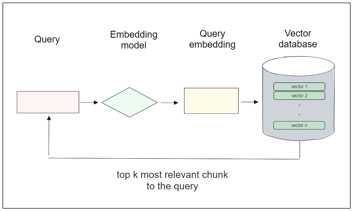
A special data structure called an index is built on top of each embedding inside a vector database during the storing process to facilitate efficient searching and retrieval of similar embeddings.

Several indexing strategies can be applied to fit our specific use case. In general, there are four categories of indexing strategies: tree-based, graph-based, hash-based, and quantization-based indexing.

Each method has its own pros and cons, and the following table is our handy index cheat sheet to help you make your choice.


Category	Index	Accuracy	Latency	Throughput	Index Time	Cost
Graph-based	Cagra (GPU)	High	Low	Very High	Fast	Very High
	HNSW	High	Low	High	Slow	High
	DiskANN	High	High	Mid	Very Slow	Low
Quantization-based or cluster-based	ScaNN	Mid	Mid	High	Mid	Mid
	IVF_FLAT	Mid	Mid	Low	Fast	Mid
	IVF + Quantization	Low	Mid	Mid	Mid	Low

Figure One: An Index Cheat Sheet | Zilliz

Please note: Not included in the table are FAISS, hash-based indexing (locality-sensitive hashing) and tree-based indexing (ANNOY).

In the following section, we’re going to discuss index algorithms supported by Milvus that are based on these four categories.

Popular Index Types Supported by Milvus

Milvus supports several indexing algorithms that you can choose based on your specific use case. Let's begin with the most basic one, known as the FLAT index.

FLAT Index

The FLAT index is a straightforward and elementary similarity search algorithm that utilizes the k-nearest neighbors (kNN) algorithm.

Consider a database with a collection of 100 embeddings and a query embedding Q. To find the most similar embedding to Q, kNN calculates the distance between Q and each embedding in the database using a specified distance metric. It then identifies the embedding with the smallest distance as the most similar to Q.

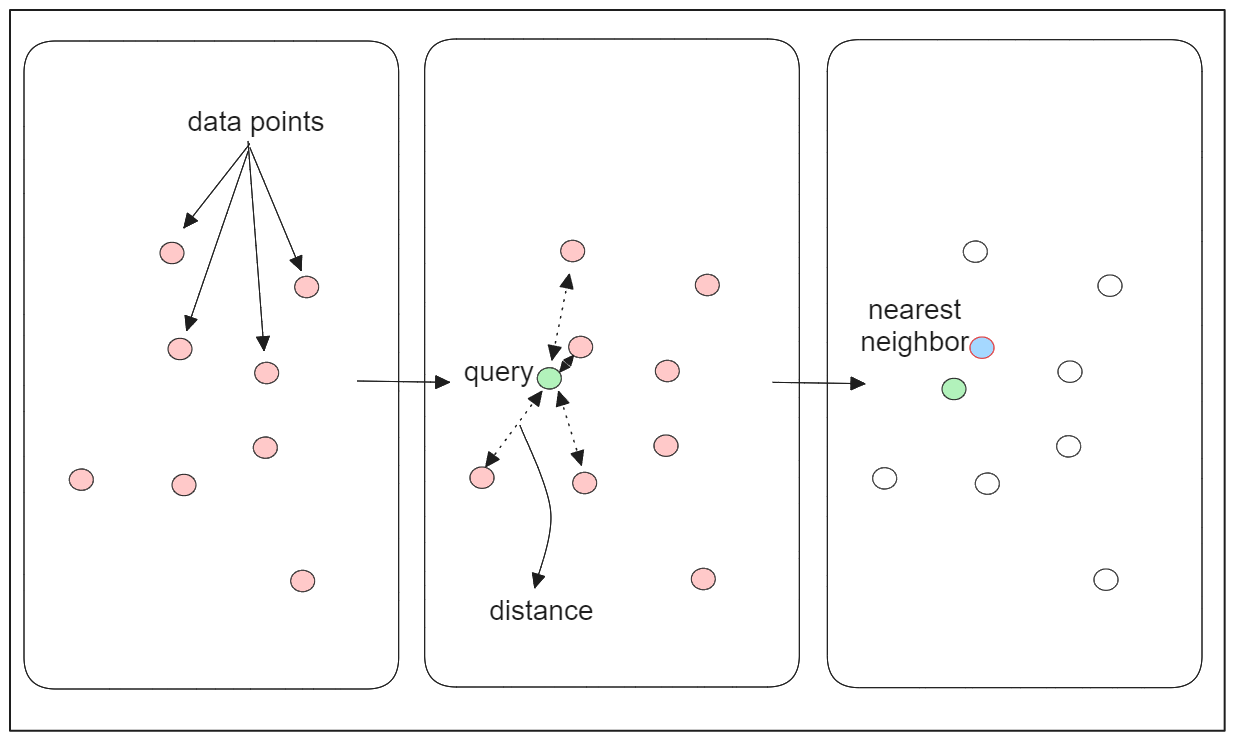
While kNN ensures high accuracy in results through exhaustive search, its scalability is a concern. The time complexity of vector search using this algorithm increases linearly with the number of vector embeddings in the database.

When dealing with millions or billions of embeddings in the database, executing vector search using this method can be time-consuming. Also, this approach lacks vector compression techniques, potentially leading to issues when we’re attempting to store millions of embeddings that may not all fit in RAM.

Inverted File FLAT (IVF-FLAT) Index

The Inverted File FLAT (IVF-FLAT) index aims to improve the search performance of the basic FLAT index by implementing approximate nearest neighbors (ANNs) algorithm instead of the native kNN. IVF_FLAT works by dividing the embeddings in the database into several non-intersecting partitions. Each partition has a center point called a centroid, and every vector embedding in the database is associated with a specific partition based on the nearest centroid.

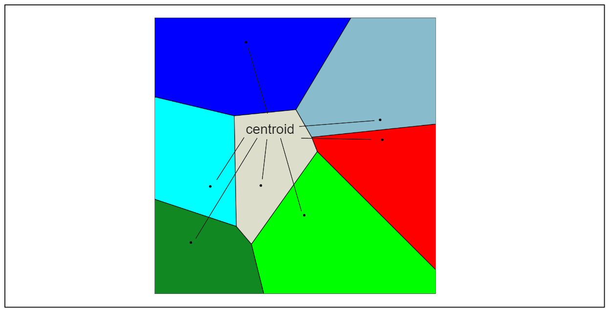
When a query embedding Q is provided, IVF-FLAT only needs to calculate the distance between Q and each centroid rather than the entire set of embeddings in the database. The centroid with the smallest distance is then selected, and the embeddings associated with that partition are used as candidates for the final search.

This indexing method speeds up the search process, but it comes with a potential drawback: the candidate found as the nearest to the query embedding Q may not be the exact nearest one. This can happen if the nearest embedding to Q resides in a partition different from the one selected based on the nearest centroid (see visualization below).

To address this issue, IVF-FLAT provides two hyperparameters that we can tune:

nlist: Specifies the number of partitions to create using the k-means algorithm.
nprobe: Specifies the number of partitions to consider during the search for candidates.

Now if we set nprobe to 3 instead of 1, we get the following result:

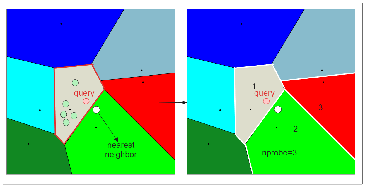
By increasing the nprobe value, you can include more partitions in the search, which can help ensure that the nearest embedding to the query is not missed, even if it resides in a different partition. However, this comes at the cost of increased search time, as more candidates need to be evaluated.

Inverted File Index with Quantization (IVF-SQ8 and IVF-PQ)

The IVF-FLAT indexing algorithm mentioned earlier accelerates the vector search process. However, when memory resources are limited, using the FLAT strategy may not be optimal as it does not compress the values of the embeddings.

To address memory constraints, an additional step can be combined with IVF, which involves mapping the values in each vector dimension to lower-precision integer values. This mapping strategy is commonly known as quantization, and there are two main quantization approaches: scalar quantization and product quantization.

Inverted File Index and Scalar Quantization (IVF-SQ8)

Scalar quantization involves mapping floating-point numbers representing each vector dimension to integers.

In scalar quantization, the first step is to determine and store the maximum and minimum values of each dimension of the vectors in the database to calculate the step size. This step size is crucial for scaling the floating-point number in each dimension to its integer representation. For example, converting a 32-bit floating-point number to an 8-bit integer typically involves splitting the range into 256 buckets. The step size can be calculated as: step size formula.png

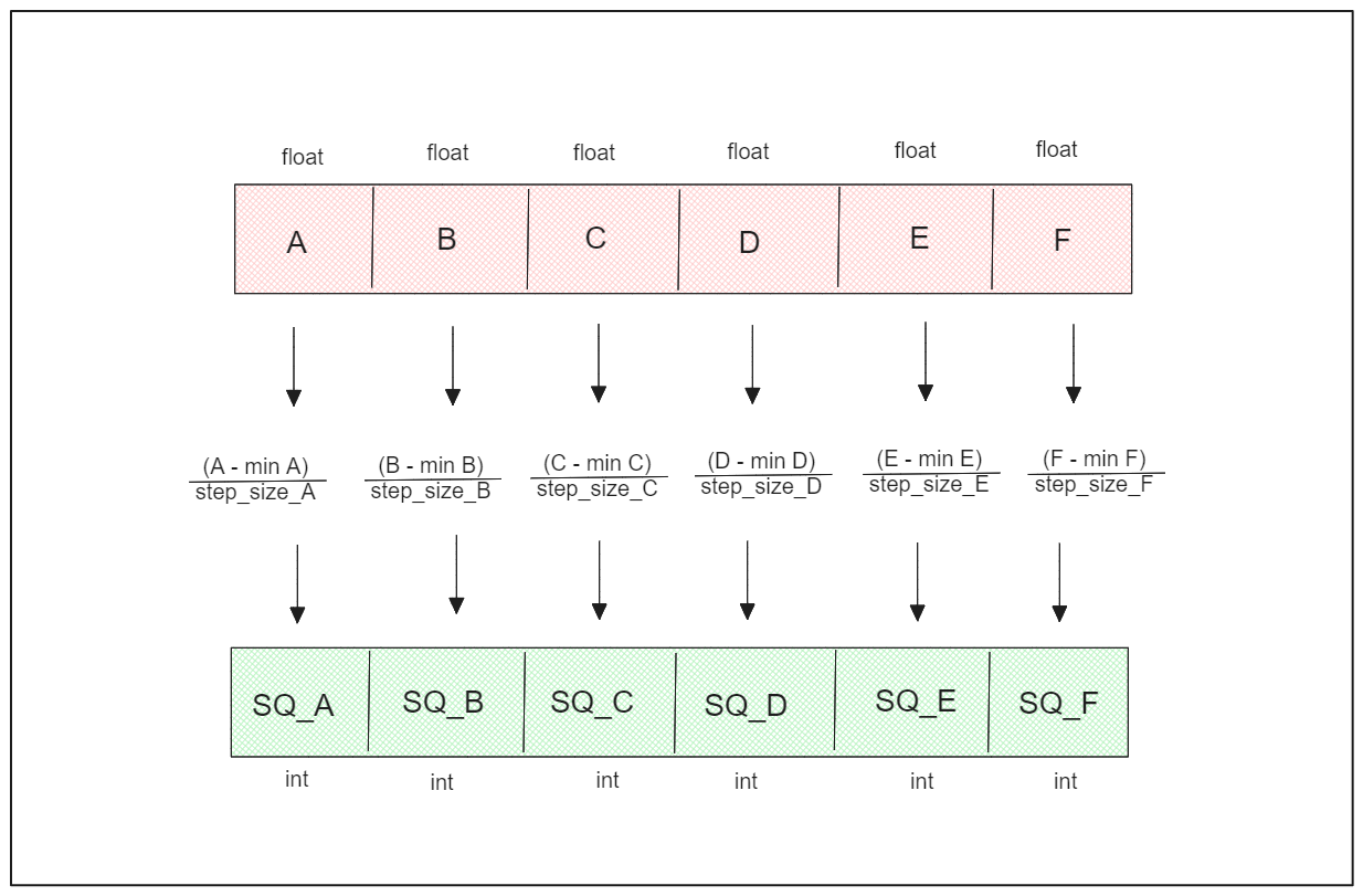
The quantized version of the n-th vector dimension is obtained by subtracting the value of the n-th dimension from its minimum value and then dividing the result by the step size.

Inverted File Index and Product Quantization (IVF-PQ)

Product quantization addresses the limitation of scalar quantization by considering the distribution of each dimension.

Product quantization divides vector embeddings into subvectors, performs clustering within each subvector to create centroids, and encodes each subvector with the ID of the nearest centroid. This method creates non-intersecting partitions within subvectors, similar to IVF-FLAT.

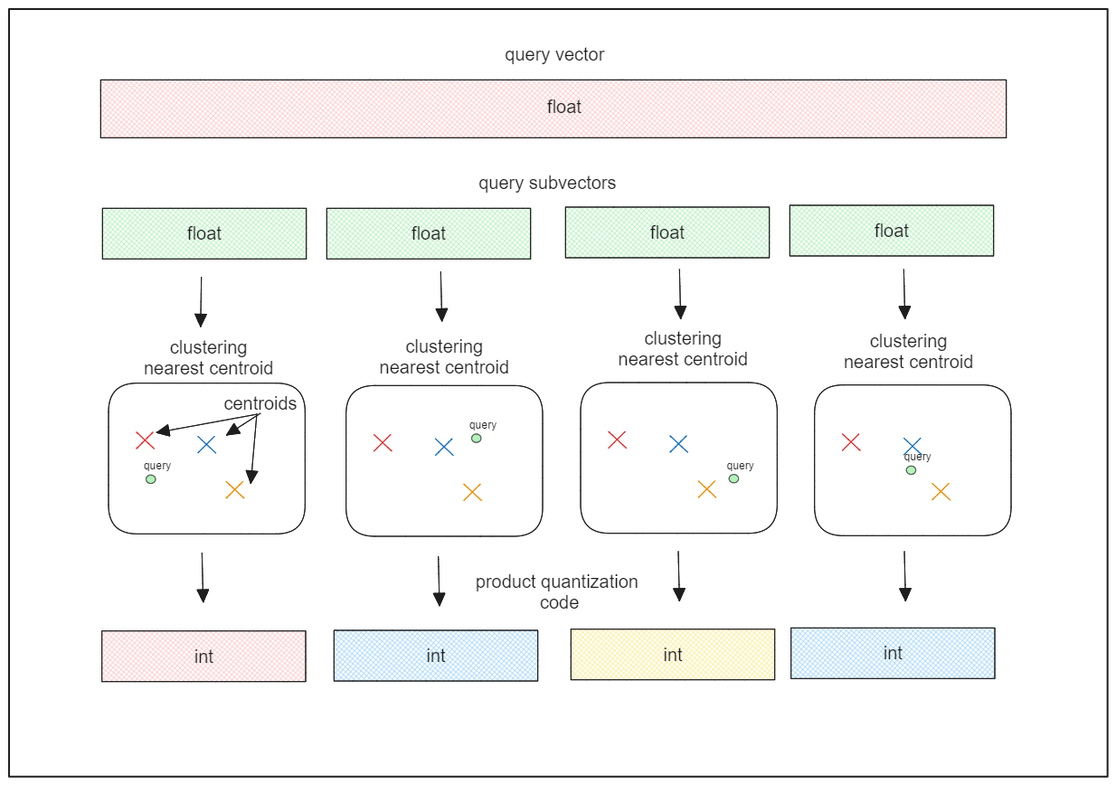
The ID of the centroid, known as the PQ code, represents an 8-bit integer, resulting in memory-efficient encoding of vector embeddings.

Product quantization offers more powerful memory compression compared to scalar quantization, making it a highly useful method for handling massive memory constraints in similarity search applications.

Hierarchical Navigable Small World (HNSW)

HNSW is a graph-based indexing algorithm that combines two key concepts: skip lists and Navigable Small World (NSW) graphs.

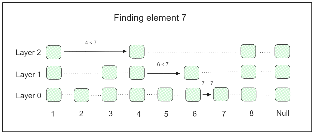
A skip list is a probabilistic data structure composed of multiple layers of linked lists. The lowest layer contains the original linked list with all elements. As we move to higher layers, the linked lists progressively skip over more elements, resulting in fewer elements at each higher layer.

During the search process, we start from the highest layer and gradually descend to lower layers until we find the desired element. Because of this, skip lists can significantly speed up the search process.

Let’s say we have a skip list with 3 layers and 8 elements in the original linked list. If we want to find element 7, the searching process will look something like this:

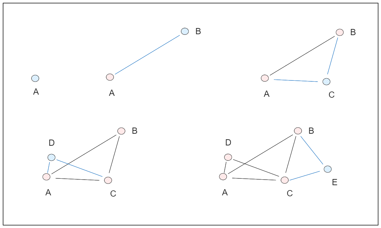
On the other hand, an NSW graph is built by randomly shuffling data points and inserting them one by one, with each point connected to a predefined number of edges (M). This creates a graph structure that exhibits the "small world" phenomenon, where any two points are connected through a relatively short path.

As an example, let’s say we have 5 data points and then we set the M=2. The step-by-step process of building an HSW graph is shown below:

The "Hierarchical" terms in HNSW refers to the combination of the skip list and NSW graph concepts. HNSW consists of a multi-layered graph, where the lower layers contain the complete set of data points, and the higher layers contain only a small fraction of the points.

HNSW starts by assigning a random integer number from 0 to l to each data point (can be referred to as “node”—as we call it in graph algorithm), where l is the maximum layer at which that data point can be present in a multi-layered graph. If a data point has l=2 and the total number of layers in the graph is 5, then that data point should only be present up until the second layer, and shouldn’t be available in layer 3 upwards.

During the search process, HNSW starts by selecting an entry point, and this should be the data point present in the highest layer. It then searches for the neighbor closest to the query point and recursively continues the search in lower layers until the nearest data point is found.

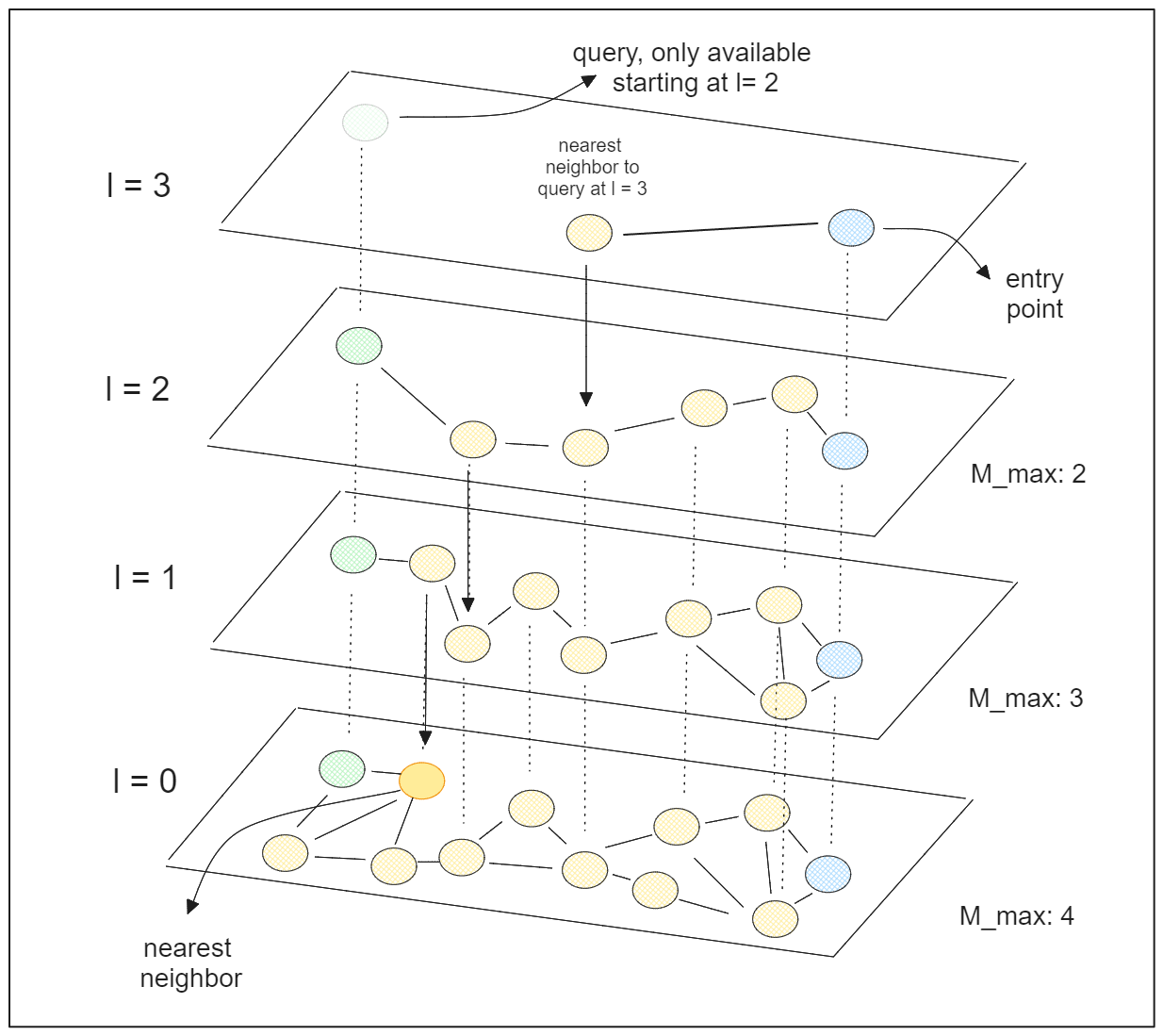
HNSW has two key hyperparameters that we can tune to improve search accuracy:

efConstruction: The number of neighbors considered to find the nearest neighbor at each layer. Higher values result in more thorough searches and better accuracy, but with increased computation time.
efSearch: The number of nearest neighbors to consider as the entry point in each layer.

By leveraging the concepts of skip lists and NSW graphs, HNSW can significantly speed up the similarity search process by skipping over many unpromising data points.

Which Index Types to Use?

We now know different index types supported by Milvus. Understanding the various index types supported by Milvus is crucial, but the decision on which index type to use depends on your specific use case and the objectives of your similarity search.

Considerations such as the importance of the accuracy of results, query speed, memory constraints, and data size play a significant role in selecting the appropriate index type. To hel you decide the index types for your use case, refer to the following flowchart:

For precise searches that guarantee 100% accuracy, the FLAT index is the ideal choice. However, if speed is a priority and exact accuracy is not that critical, other indexing algorithms can be selected.

If memory resources are a concern, consider using quantized indexing algorithms like IVF-SQ8 or IVF-PQ. Otherwise, options like IVF-FLAT or HNSW can be suitable. For smaller datasets (less than 2GB), IVF-FLAT may suffice, while larger datasets (over 2GB) can benefit from HNSW for improved search speed, whilst still maintaining high recall.

In cases of exceptionally large datasets, combining IVF with a quantization method remains a preferred approach to prevent memory overload.

Conclusion

Selecting the right index type for storing vector embeddings is crucial for achieving the desired search results. Each index type has its own strengths and considerations, making the choice dependent on the specific requirements of your use case.

For further insights into the indexing methods discussed in this article, explore the additional resources provided by us.