


Understanding Latent Semantic Analysis (LSA)

Understanding Latent Semantic Analysis (LSA)
TL;DR
Latent Semantic Analysis (LSA) is a natural language processing (NLP) technique used to uncover relationships between terms and documents in a text corpus. It reduces high-dimensional text data into a lower-dimensional representation by applying Singular Value Decomposition (SVD) to the term-document matrix. This process captures the latent semantic structure of the data, grouping similar words and documents based on their contextual meanings. LSA is commonly used in tasks like document clustering, information retrieval, and topic modeling. By revealing hidden patterns in the data, LSA improves the understanding and organization of large text datasets.

Introduction
Have you ever wondered how search engines understand what you’re looking for, even when you don’t use the exact words? That’s where Latent Semantic Analysis (LSA) comes in.
LSA identifies the underlying connections between words by recognizing patterns and relationships in text. For example, when you search for “best running shoes,” you might get results on shoe brand comparisons, shoe reviews, and even running tips. All of these are relevant to your search, even though the exact words you used aren’t present. LSA makes it possible by recognizing patterns in text and uncovering relationships between words. This helps systems like search engines, recommendation algorithms, and AI-powered chatbots understand the context and meaning, not just keywords.
Now, let's see in detail what LSA is, how it works, its importance, benefits, challenges, and applications.
What is LSA?
Latent Semantic Analysis is a Natural Language Processing (NLP) method that uses mathematical techniques like Singular Value Decomposition (SVD) to identify associations and contextual meanings of words within large bodies of text.
The origins of LSA date back to the late 1980s. It was first applied to uncover hidden semantic structures in text. In 1988, Scott Deerwester and colleagues patented a technique for information retrieval. This technique was based on a latent semantic structure called Latent Semantic Indexing (LSI). It was groundbreaking because it allowed systems to retrieve relevant documents without exact keyword matches at a time when keyword matching was the primary method for information retrieval. Instead, it relied on the underlying semantic connections between terms.
You can think of LSA as a smart librarian who notices hidden patterns in text and connects words and ideas in a meaningful way.
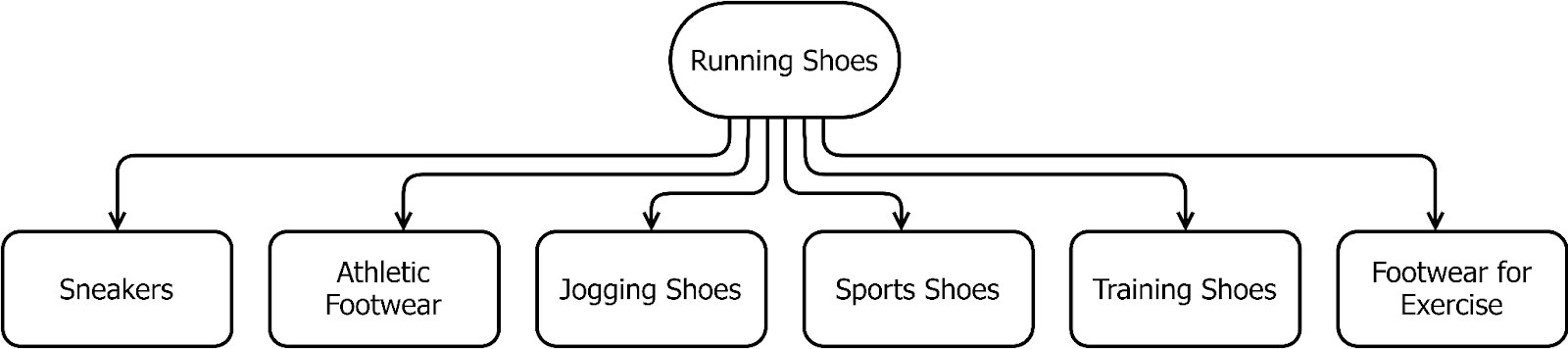 Figure- Running Shoes Semantic Network
Figure: Running Shoes Semantic Network
With LSA, systems can:
Find hidden relationships between words and ideas
Understand text better and improve information retrieval
Improve search results by connecting related terms
Find deeper meanings in large text collections
LSA is an unsupervised learning approach that does not require labeled data to uncover relationships and structures within the text. It uses singular value decomposition (SVD) to reduce the dimensionality of the term-document matrix, transforming it into a smaller set of latent features. These features capture the most significant patterns in the data, highlighting the underlying semantic relationships.
How Does LSA Work?
LSA involves four steps. We will go over the implementation of each step using the Python library scikit-learn.
Text Preprocessing
Document-Term Matrix Creation
Singular Value Decomposition (SVD)
Topic-Encoded Data
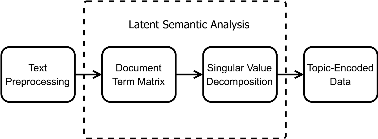 Figure- Step-by-Step Breakdown of LSA.png
Figure: Step-by-Step Breakdown of LSA
Text Preprocessing
We prepare our raw text data as documents stored as strings in a list.
documents = [
"tall green tree sway",
"short green bush stand",
"tall yellow tree glow",
"short yellow flower bloom”
]
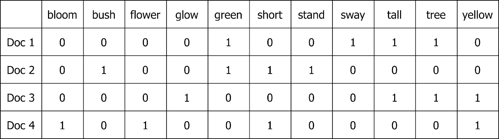 Figure- The Document-Term Matrix.png
Document-Term Matrix
A document-term matrix represents frequencies of terms appearing in the text document collection.
Figure: The Document-Term Matrix
This document-term matrix can be generated using the CountVectorizer model in scikit-learn.
from sklearn.feature_extraction.text import CountVectorizer
vectorizer = CountVectorizer()
document_term_matrix = vectorizer.fit_transform(documents)
This process transformed each document into a vector.
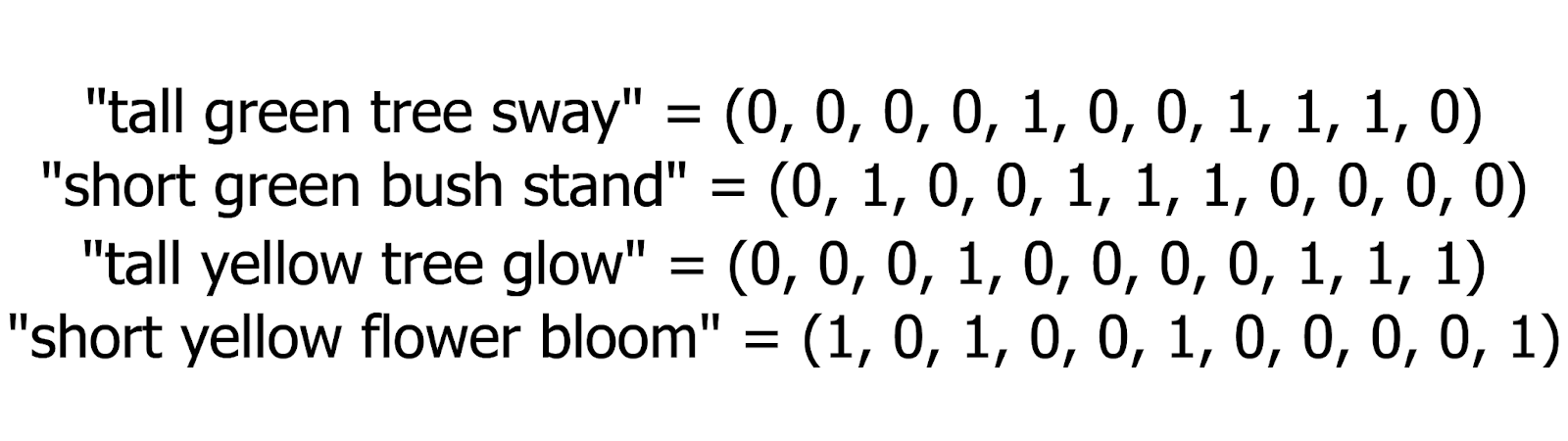 Figure- Documents to Vectors.png
Figure: Documents to Vectors
We can use document_term_matrix.todense() to view our document-term matrix.
document_term_matrix.todense()
Output:
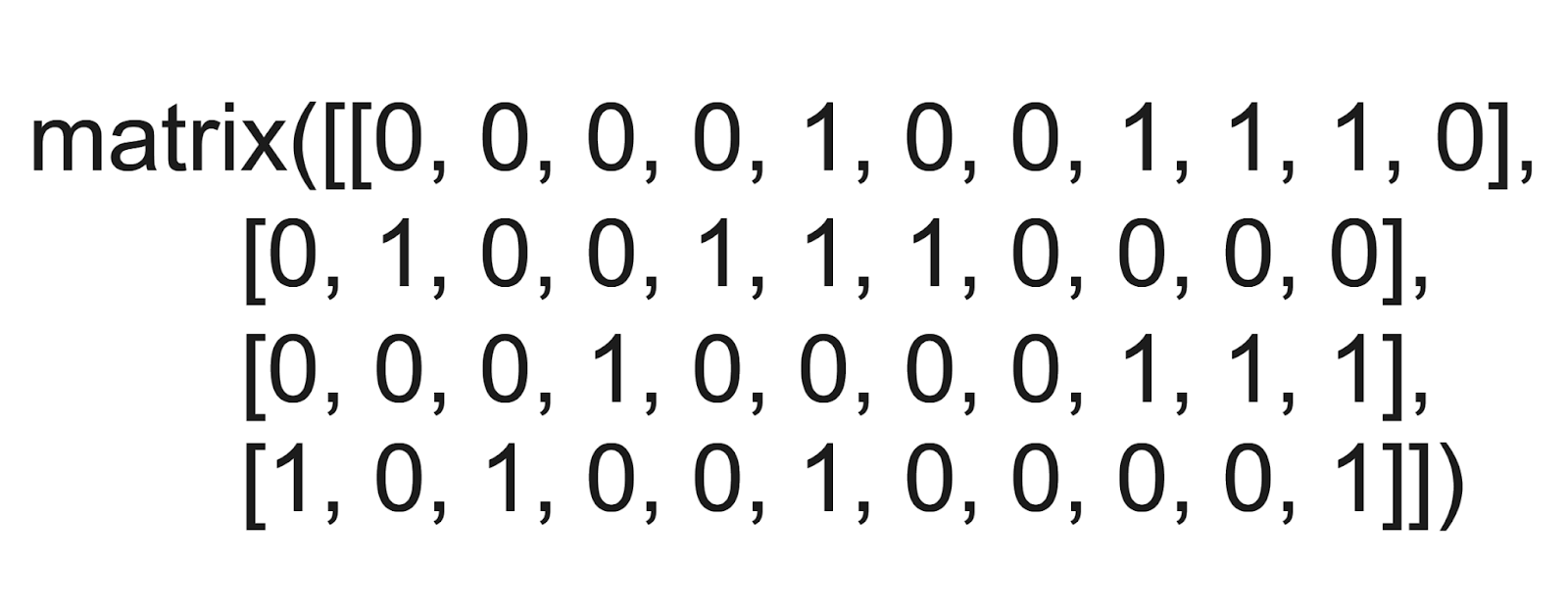 Figure- The Output
Figure: The Output
The resulting matrix shows each row as a vector. Each row corresponds to a document, and the columns represent the terms. The values indicate how many times each term appears in each document.
Singular Value Decomposition
SVD is a mathematical technique used to simplify complex datasets. SVD decomposes a matrix A into three separate matrices:
_A=UΣVT_
A: __A document-term matrix representing documents and their term frequencies.
U: An orthogonal document-topic matrix showing how strongly each document relates to each topic.
Σ: A diagonal singular values matrix capturing the importance of topics.
_VT_: An orthogonal term-topic matrix showing relationships between the terms and topics.
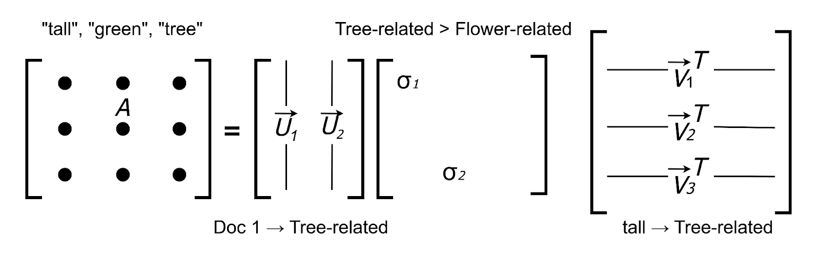 Figure- SVD in Our Use Case
Figure: SVD in Our Use Case
Dimensionality Reduction with Truncated SVD
Dimensionality reduction is an inherent capability of SVD. The technique simplifies datasets by reducing the number of features while retaining the most important information.
SVD can be achieved using the TruncatedSVD model in scikit-learn. It is called “truncated” SVD because it reduces the number of features in the dataset without significant loss of information. This makes it an effective tool for dimensionality reduction.
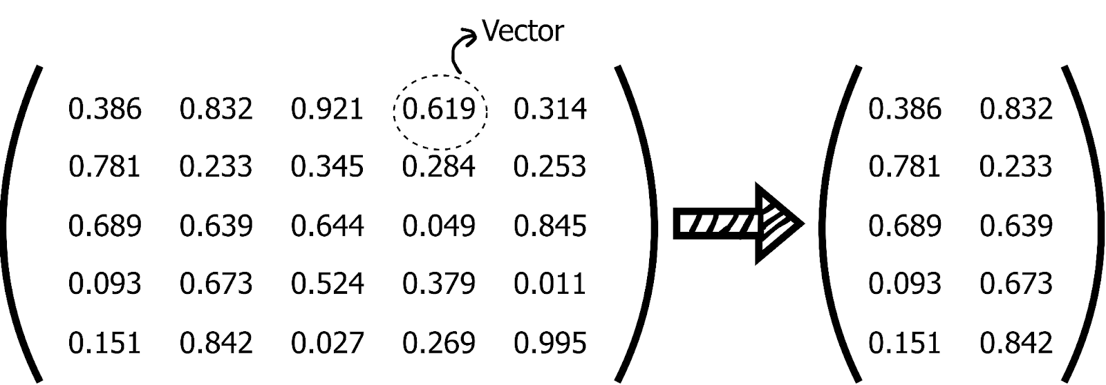 Figure- Dimensionality Reduction
Figure: Dimensionality Reduction
We will create an SVD model to fit and transform our document-term matrix.
from sklearn.decomposition import TruncatedSVD
svd = TruncatedSVD(n_components=2)
lsa = svd.fit(document_term_matrix)
This process prepares our model to transform the original data into topic-encoded data. We set n_components=2 in TruncatedSVD to represent two topics. A topic represents words that frequently appear together across documents.
In our case, a topic captures a recurring theme related to trees and plants. Words like "tall," "green," and "tree" appear together, which shows underlying patterns in the data. Thus, SVD compresses the data and reveals its semantic structure.
Topic-Encoded Data
The data now contains two columns. Each column represents one of the two topics we specified in the TruncatedSVD. We use the pandas library to see the output of our LSA.
import pandas as pd
lsa_transformed = svd.transform(document_term_matrix)
topic_df = pd.DataFrame(lsa_transformed, columns=["Topic 1", "Topic 2"])
topic_df["Original Document"] = documents
print(topic_df[["Original Document", "Topic 1", "Topic 2"]].to_string(index=False))
Output:
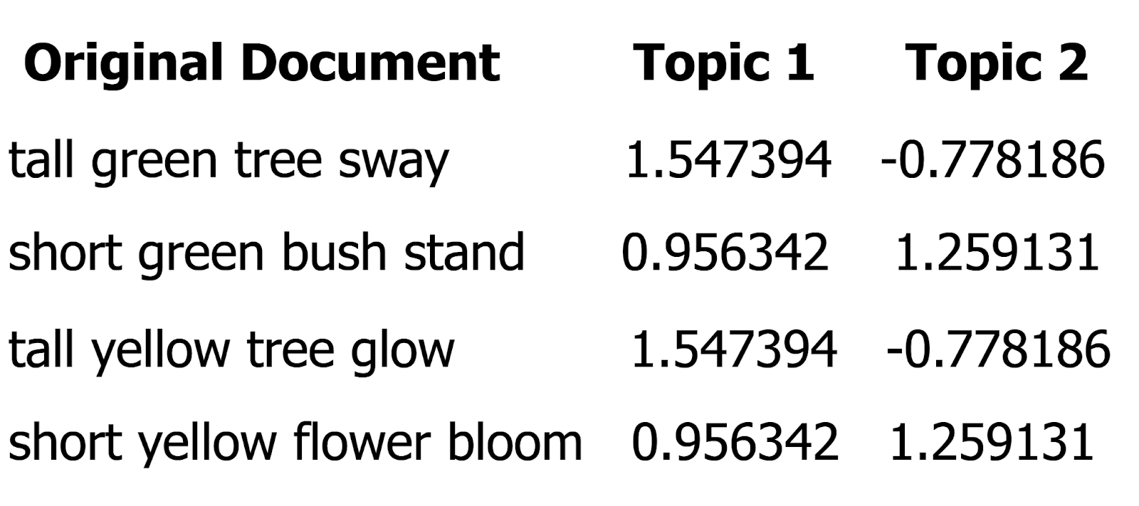
Figure: The Output
The output shows the original four documents alongside numerical values. The values represent how strongly each document is associated with the two topics. We observe that all four documents are strong in Topic 1. However, there is a clear difference in Topic 2, where:
The first and third documents are negative.
The second and fourth documents are positive.
This suggests that the first and third documents focus on tall trees, while the second and fourth are about short bushes and flowers. This numerical representation helps clearly distinguish themes in the text based on the topics.
We can take it a step further by understanding what each topic represents through the dictionary and encoding matrix.
A dictionary is a collection of all unique words in the documents.
An encoding matrix shows how strongly each word relates to each topic.
Viewing the Dictionary
The dictionary is part of the CountVectorizer model, accessible through the .get_feature_names_out() method.
vocabulary = vectorizer.get_feature_names_out()
print("Dictionary:", vocabulary)
**Output:

Figure: The output
These words form the foundation for analyzing how topics are constructed.
Viewing the Encoding-Matrix
The encoding matrix is stored as components_ in the TruncatedSVD model. It provides a mapping of words to topics.
encoding_matrix = pd.DataFrame( svd.components_.T, index=vocabulary, columns=["Topic 1", "Topic 2"] ) print(encoding_matrix)
Output:
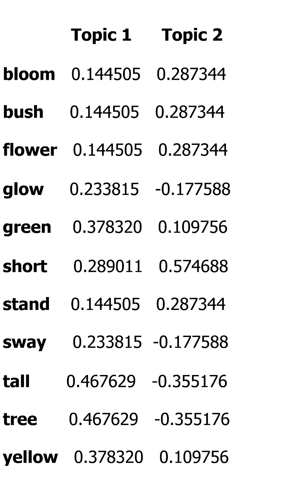
Figure: The output
Each row corresponds to a word, and each column corresponds to a topic. The values indicate how strongly a word is associated with each topic.
Interpreting the Encoding Matrix
We focus on the absolute values of the encoding to identify the most important words for each topic.
encoding_matrix["Abs Topic 1"] = encoding_matrix["Topic 1"].abs()
encoding_matrix["Abs Topic 2"] = encoding_matrix["Topic 2"].abs()
topic_1_top_words = encoding_matrix.sort_values("Abs Topic 1", ascending=False)
topic_2_top_words = encoding_matrix.sort_values("Abs Topic 2", ascending=False)
print("Top Words for Topic 1:")
print(topic_1_top_words[["Topic 1"]].head())
print("Top Words for Topic 2:")
print(topic_2_top_words[["Topic 2"]].head())
Output:
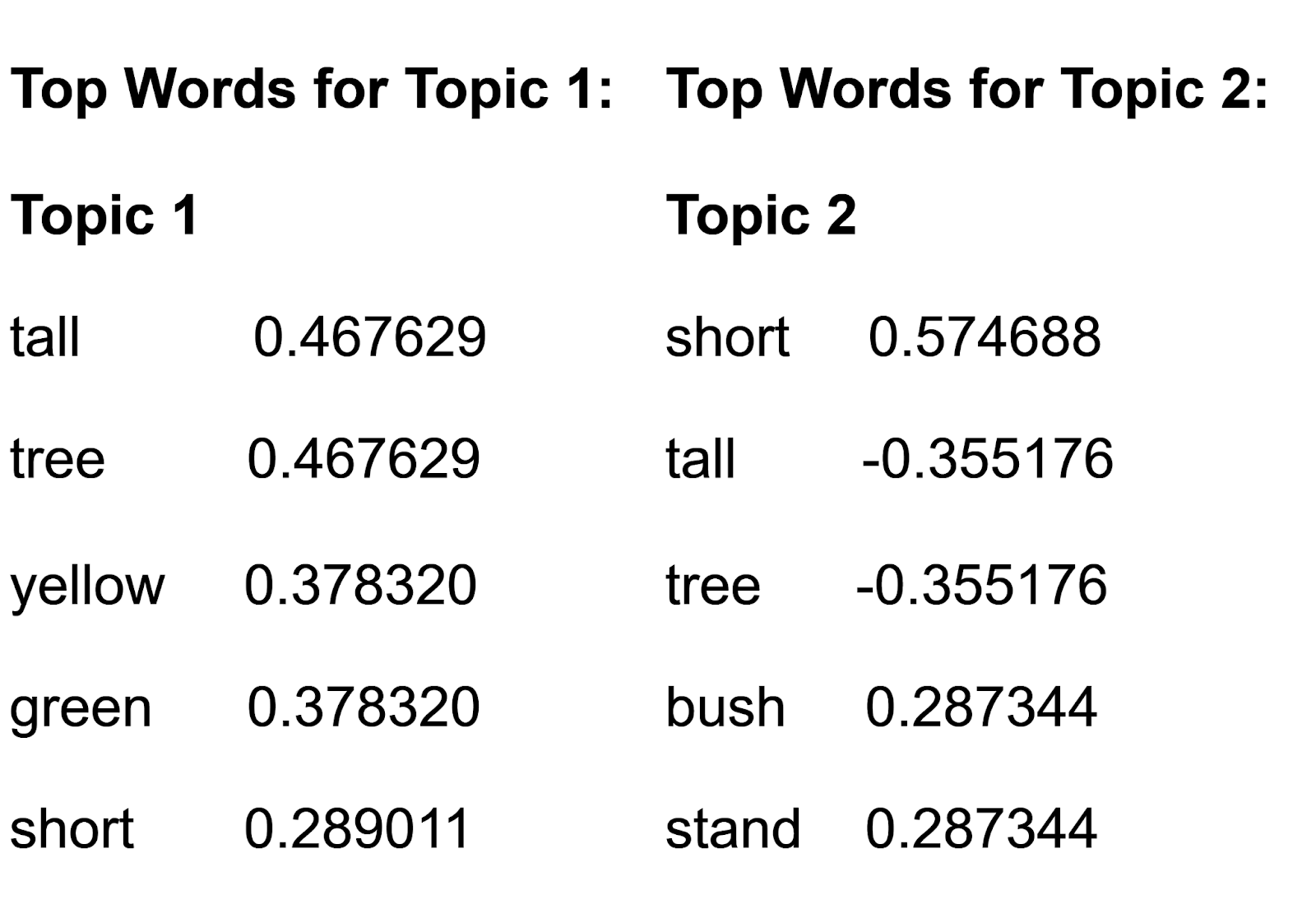 Figure- the output 4.png
Figure: the output
We observe that:
For Topic 1, words like "tall" and "tree" are important.
For Topic 2, words like "short" and "tall" are important.
Topic 2 contrasts with the words "short," which has a positive value, and "tall," which has a negative value. This shows that Topic 2 is suitable for distinguishing whether a given document is “short” or “tall.” These words' strong positive and negative values indicate their significance within this topic. Since Topic 2 has a positive value for the word “short,” we can use this topic to tell how closely a given document relates to “short.”
Comparison with Similar Techniques
LSA is often compared to other similar techniques in text analysis. Here's a comparison to clarify common misconceptions:
LSA vs. LDA
LDA (Latent Dirichlet Allocation) is a probabilistic model that generates topics by assuming a hierarchical Bayesian distribution. Meanwhile, LSA uses SVD to reduce the dimensionality of the term-document matrix. This makes LSA a deterministic method because it uses fixed transformations (SVD), giving the same result every time for the same input.
LDA provides probabilities for words within topics and topics within documents. It creates more coherent topics due to its probabilistic framework. This makes it better for large and noisy datasets. On the other hand, LSA is effective for smaller datasets and exploring semantic relationships.
LSA vs. NMF
NMF (Non-negative Matrix Factorization) shares similarities with LSA in its use of matrix factorization. However, it imposes a non-negativity constraint, ensuring all components are additive. This constraint makes NMF results more interpretable than LSA, which allows negative values in its factorization process.
For example, the topics identified by NMF will only show positive associations between terms like "good" and "quality" in a positive review. This makes NMF easier to interpret. Another distinction lies in the consistency of the results. LSA gives the same output due to its use of SVD. NMF's results can vary depending on initialization and often require multiple runs for optimization.
Benefits and Challenges of LSA
Understanding the benefits and challenges of LSA is essential for effectively applying it in natural language processing tasks.
Benefits
Some of the key benefits of LSA include:
Improved Information Retrieval: LSA improves search engine accuracy by considering the semantic meaning of words. This allows for more relevant search results.
Dimensionality Reduction: LSA simplifies complex data by reducing the number of dimensions in the document-term matrix. This makes the data more manageable and interpretable.
Semantic Analysis: LSA captures latent semantic relationships between terms and documents. This helps in tasks like document clustering and topic modeling.
Challenges
Some of the challenges associated with LSA include:
Assumption of Linear Relationships: LSA assumes linear relationships between terms and concepts. This may not always align with the true nature of language. As a result, it can lead to inaccuracies, such as misinterpretations of word meanings.
Order of Words: LSA does not account for the order of words in a document, which can be crucial for understanding context and meaning.
Handling of Synonyms and Polysemy: LSA may struggle with words with multiple meanings (polysemy) or synonyms. It doesn't explicitly disambiguate these terms.
Applications, Tools, and Providers of LSA
LSA has broad applicability in NLP and information retrieval, and it is supported by various tools and platforms that enhance its integration and scalability.
Applications
LSA is widely used in real-world applications within NLP and information retrieval systems. These include:
Search Engines: LSA helps improve search results by identifying latent semantic structures in documents and queries.
Recommendation Systems: LSA suggests relevant items by analyzing the semantic relationships between users and items based on historical data or preferences.
Document Clustering: LSA reduces dimensionality and uncovers semantic relationships. This allows it to automatically group similar documents together, helping to organize large text corpora.
Chatbots/NLP Applications: LSA enhances chatbots and other NLP applications by improving the understanding of context and intent.
Tools
Various tools support the implementation of LSA:
Milvus: An open-source vector database for storing and querying vector embeddings converted by LSA techniques to perform semantic similarity searches.
scikit-learn: A Python library providing utilities for generating LSA embeddings through techniques like SVD.
Gensim: A Python library widely used for topic modeling and document similarity analysis. Gensim provides an efficient implementation of Latent Semantic Indexing (LSI) through its gensim.models.LsiModel class.
Connection to Milvus
Milvus enables efficient storage and retrieval of embeddings. It is ideal for performing fast and accurate vector similarity searches.
Workflow Overview
The process involves:
Embedding Generation: We use DefaultEmbeddingFunction to convert documents like "tall green tree sway" into vector representations. These embeddings are crucial for performing semantic similarity searches.
Storage in Milvus: Store the generated embeddings along with associated metadata in Milvus for efficient management.
Similarity Search: A query vector is generated from a search phrase like "tall green tree sway." This vector is used to search the collection for the most similar matches.
Connection to Milvus
Milvus enables efficient storage and retrieval of embeddings. It is ideal for performing fast and accurate vector similarity searches.
Workflow Overview
The process involves:
Embedding Generation: We applied LSA to transform documents like "tall green tree sway" into vector representations. These vectors encapsulate the semantic structure of the text.
Storage in Milvus: Store the transformed vectors along with associated metadata in a Milvus collection.
Similarity Search: Use a query vector like "tall green tree sway" to retrieve the most semantically similar documents from the collection.
Steps to Follow
Create a Milvus Collection: Initialize a collection specifying the vector dimension.
Insert Data: Add the LSA-transformed vectors and their metadata into the collection.
Perform Similarity Search: Query the collection using a vector to find the closest matches.
from pymilvus import MilvusClient

client = MilvusClient(
    uri="http://localhost:19530",
    token="root:Milvus",
    db_name="default"
)

if client.has_collection(collection_name="coll"):
    client.drop_collection(collection_name="coll")
client.create_collection(
    collection_name="coll",
    dimension=2,
)

vectors = lsa_transformed

data = [
    {"id": i, "vector": vectors[i], "document": documents[i]}
    for i in range(len(vectors))
]
data

res = client.insert(collection_name="coll", data=data)

query_vectors = [lsa_transformed[0]]

res = client.search(
    collection_name="coll",
    data=query_vectors,
    limit=3,
    output_fields=["document"],
)

for item in res[0]:
    print(f"ID: {item['id']}")
    print(f"Distance: {item['distance']}")
    print(f"Entity:")
    print(f"  Document: {item['entity']['document']}\n")
Output:
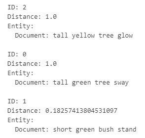
We have retrieved the most relevant documents based on their semantic closeness.
FAQs
- How does LSA handle polysemy, and what are its limitations?
LSA treats each word as having a single meaning. This leads to issues with polysemous words, which cause semantic inaccuracies.
- What are the computational challenges with LSA on large datasets?
LSA requires SVD, which is computationally intensive and time-consuming, especially with large datasets. Moreover, the dimensions produced by SVD can be difficult to interpret.
- What are the limitations of LSA in capturing word order?
LSA ignores word order, which affects tasks like sentiment analysis, where word sequence (e.g., "not good" vs. "good not") influences meaning.
- How does LSA handle synonyms, and what challenges arise?
LSA identifies latent semantic relationships between words. However, it can struggle with subtle differences between synonyms, complicating tasks like document clustering.
- How does LSA deal with sparsity in term-document matrices?
LSA creates sparse term-document matrices, which can reduce accuracy and efficiency. Even with SVD, this sparsity limits its performance in tasks like document classification.
Related Sources
- TL;DR
- Introduction
- What is LSA?
- How Does LSA Work?
- Comparison with Similar Techniques
- Benefits and Challenges of LSA
- Applications, Tools, and Providers of LSA
- FAQs
- Related Sources
Content
Start Free, Scale Easily
Try the fully-managed vector database built for your GenAI applications.
Try Zilliz Cloud for Free