Improving Analytics with Time Series and Vector Databases
Time series analysis plays a crucial role in many fields, particularly in Internet of Things (IoT) devices. With time series data, we can detect patterns and trends over particular periods, enabling us to forecast and analyze future time-dependent events. Common examples of time series use cases include forecasting weather temperatures and stock prices and monitoring sensor data.
As a time series database, InfluxDB provides a solution for storing vast amounts of time series data. InfluxDB is highly optimized for storing and querying time-dependent data using techniques such as aggregations and downsampling. However, relying on time-series databases alone can be challenging, especially if our use case demands us to perform a similarity search.
In a recent talk at the Zilliz Unstructured Data Meetup, Zoe Steinkamp, Developer Advocate at InfluxDB, discussed an approach to combining InfluxDB with Milvus to store, query, and perform similarity searches on time-dependent use cases.
In this article, we'll explore this topic in more detail and walk you through a use case where we'll store time-series data in InfluxDB, query the data, transform it into vector embeddings, store the embeddings in Milvus, and finally perform a similarity search with Milvus. So, without further ado, let's get started.
Understanding Time Series Data
Time series data represents chronologically ordered observations recorded at specific intervals, such as hourly, daily, weekly, or monthly.
We can find time series use cases in our everyday life: from hourly temperature readings, daily road traffic statistics, to monthly retail sales figures. By analyzing time series data, we can uncover historical patterns and use these insights to inform future decisions.
When analyzing time series data, we often see one or more of the following patterns:
Seasonal: Recurring fluctuations at fixed time intervals, influenced by factors like weekdays or months.
Trend: A steady increase or decrease in the data over an extended period.
Cyclic: Fluctuations similar to seasonal patterns, but without a fixed frequency.
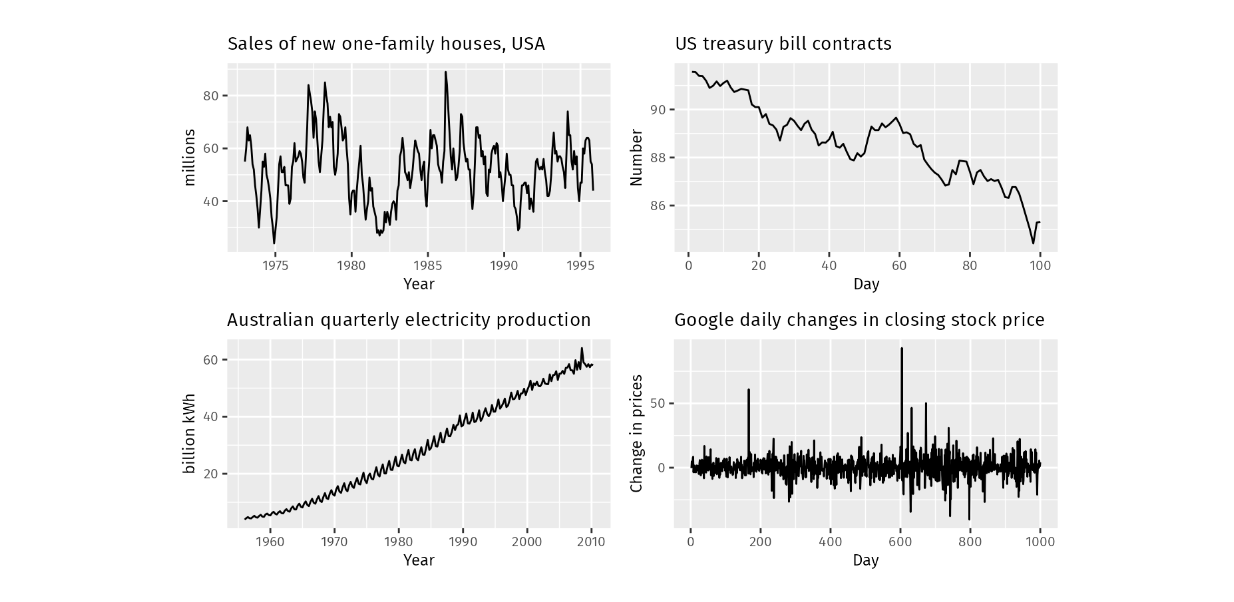
Top left - seasonal, top right -decreasing trend, bottom left - increasing trend, bottom right - cyclic. Source.
Understanding these patterns is crucial for effective time series forecasting. Time series forecasting is a powerful analytical technique that predicts future values of time-dependent variables based on historical data. For example, if we have a stock's price history for the previous two years and want to predict tomorrow's stock price, we're essentially performing time series forecasting.
Companies across different sectors have applied the concept of time series forecasting in their daily operations for various purposes:
Financial Institutions: Predicting stock prices, forecasting currency fluctuations, identifying unusual patterns in customer spending, or developing robust risk management strategies.
Healthcare Sector: Monitoring the spread of diseases, tracking patients' vital signs in real-time, or enhancing overall patient care and outcomes.
Retail Industry: Forecasting sales volumes, understanding customer purchasing behaviors, optimizing inventory management, fine-tuning pricing strategies, and boosting overall profitability.
Internet of Things (IoT): Smart home systems use sensor data to automate tasks, while thermostats and home hubs exchange information to optimize energy use.
Manufacturing: Reducing machine downtime, implementing predictive maintenance strategies, and improving overall operational efficiency.
Due to its time-dependent nature, time series data is typically collected continuously in real time. As a result, the volume of time series data can grow rapidly, necessitating a scalable and efficient solution for storage. This is where time-series databases come into play.
InfluxDB as a Time Series Database
Time series databases need to possess several key characteristics compared to traditional relational databases to facilitate the storage and retrieval process of large amounts of time series data. As mentioned previously, time series data is often collected in real time; therefore, the data needs to be processed and synced across all systems as soon as it reaches the database.
Time series databases offer better performance and efficiency than relational databases for time-based workloads, especially when dealing with large volumes of data and high-frequency writes. Additionally, a time series database offers highly optimized solutions for operations such as data ingestion, querying, and retrieval over time ranges, as well as time-based analytics and aggregations.
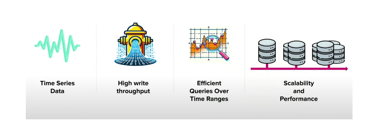 Important features in a time series database
InfluxDB is one of the open-source time series databases that we can use to store time series data. It's written in Rust, and is highly optimized for extract, transform, load (ETL) operations in databases. To facilitate fast data ingestion and timestamp synchronization, InfluxDB contains a built-in time service that uses the Network Time Protocol (NTP).
The time series data that we store inside a time series database typically consists of only three columns: a tag, a field, and a timestamp. A tag contains metadata of the data we measure, a field contains values that we further analyze, and a timestamp indicates when the data was collected.
Let's say we're storing sensor measurement data every 5 minutes. The data inside our time series would look something like the visualization below:
 Example of data stored inside a time series database
Now that we know the fundamentals of time series databases, let’s talk about vector databases!
Milvus as a Vector Database
As the name suggests, a vector database stores data (including images, texts, documents, etc.) in vectors. We transform our data into vectors using one of the many deep-learning models.
The dimension of a vector depends on the technique or deep learning model we use to generate it. For example, if we use a model called all-MiniLM-L6-v2, we'll get a vector of dimension 384. Meanwhile, if we use a model called all-mpnet-base-v2, we'll get a vector of dimension 768.
As you may be aware, a vector is not just a mathematical object; it encapsulates both magnitude and direction, carrying the semantic meaning of the text, image, or document it represents. This profound aspect of vectors is what enables them to be placed close to each other in the vector space, representing similar texts or images.
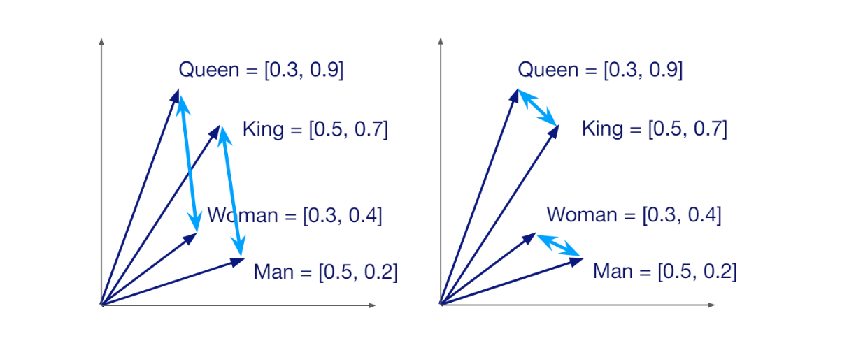 Semantic similarity between vectors in a vector space
The idea that a vector carries the semantic meaning of data enables us to compare the similarity of any pair of vectors via metrics like cosine similarity or Euclidean distance. If the cosine similarity between two vectors is close to one, then the two vectors are highly similar, and vice versa.
Storing and performing similarity searches might be simple to implement if we only have a few vectors. However, in real-life applications, we're typically dealing with hundreds of thousands or millions of vectors, which makes the entire operation more expensive to maintain in terms of both time and computational resources. This is where a vector database becomes necessary.
Vector databases like Milvus and Zilliz Cloud offer highly scalable and efficient processes for storing millions of vectors. They're also highly optimized for faster vector similarity searches and data retrieval, thanks to their wide variety of advanced indexing methods such as IVF-Flat, HNSW, and others.
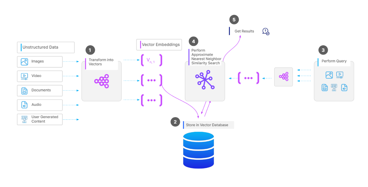 Complete workflow of a vector search operation
The workflow for storing and retrieving data from Milvus or any other vector database is as follows: First, we transform our input data, which could be texts or images, into vectors using a technique or model of our choice. Next, we ingest these vectors alongside their metadata into the vector database and build an index using an indexing method of our choice.
During the retrieval process, we first need to transform our query into a vector using the same technique or model we used during the ingestion process. Next, we perform a vector search operation to compare this query vector with the vectors stored in our vector database. Finally, the most similar vectors in the database are returned to us as results.
The Use Case of Combining Time Series Database and Vector Database
Since time series and vector databases are highly optimized for different use cases, we can leverage the strengths of both databases in our real-life projects.
For example, let's imagine a scenario where we're developing a system to analyze real-time traffic conditions in a smart city. To achieve this, we would install sensors in many locations that can track vehicle speed, vehicle count, and other relevant metrics. The average vehicle speed and vehicle count over specific time intervals could be stored continuously inside a time series database.
In addition to sensors, we could also install cameras to capture photos or videos of the actual traffic conditions. In this case, we can transform the photos and videos into vectors using a deep learning model of our choice and store these vectors in a vector database. By combining the time series data from the time series database and vectors from the vector database, we're able to perform anomaly detection on traffic conditions.
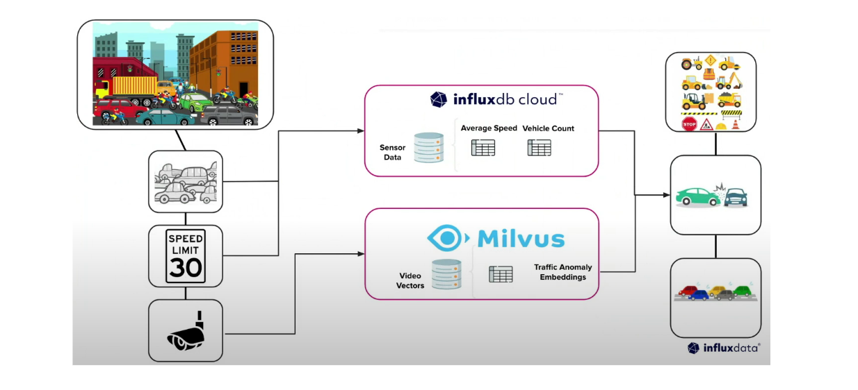 Example use case of combining InfluxDB and Milvus to analyze traffic conditions
In this section, we're going to implement a simple use case related to traffic conditions with the help of InfluxDB and Milvus. Specifically, we'll store time series data inside InfluxDB and the corresponding vectors inside Milvus.
Let's first generate dummy time series data that consists of timestamp, average vehicle speed, vehicle count, and anomaly type. The anomaly type consists of two distinct values: "normal" and "accident".
We'll start by generating 500 "normal" data points collected every 10 minutes.
import numpy as np

import pandas as pd

from datetime import datetime, timedelta

import random

def generate_sensor_data(anomaly_type, start_time, vehicle_count_range, avg_speed_range, rows=500, seed = 42):


    np.random.seed(seed)

    vehicle_counts = np.random.randint(vehicle_count_range[0], vehicle_count_range[1], size=rows)

    avg_speeds = np.random.uniform(avg_speed_range[0], avg_speed_range[1], size=rows)

    start_time = datetime.strptime(start_time, "%Y-%m-%d %H:%M:%S")

    timestamps = [start_time + timedelta(minutes=10*i) for i in range(rows)]

    df = pd.DataFrame({

        'Timestamp': timestamps,

        'Vehicle Count': vehicle_counts,

        'Average Speed': avg_speeds,

        'Anomaly Type': anomaly_type

    })

    return df


vehicle_count_range = (5, 10)

avg_speed_range = (60.0, 80.0)

df_normal = generate_sensor_data("normal", "2024-09-15 18:00:00", vehicle_count_range, avg_speed_range)
 DataFrame normal
Next, let’s generate 500 "accident" data points, also collected every 10 minutes. As you might imagine, two possible signs of an accident on the streets are a higher vehicle count and a slower average speed due to traffic congestion.
vehicle_count_range = (20, 40)

avg_speed_range = (10.0, 20.0)

df_accident = generate_sensor_data("accident", "2024-09-19 05:20:00", vehicle_count_range, avg_speed_range)
 DataFrame accident
Now let’s concatenate the two dataframe and then insert the concatenated data into InfluxDB with a command that looks like the following:
from influxdb_client_3 import InfluxDBClient3

df = pd.concat([df_accident, df_normal], axis=0)

client = InfluxDBClient3(token="DATABASE_TOKEN",

                         host="HOST",

                         database="DATABASE_NAME")

client.write(bucket="DATABASE_NAME", record=df, data_frame_measurement_name='traffic_data', data_frame_tag_columns=['Anomaly Type'], data_frame_timestamp_column='Timestamp')
And you can make a query of the data inside InfluxDB with the following command.
query = "SELECT * FROM traffic_data WHERE time >= now() - INTERVAL '90 days'"

pd = client.query(query=query, mode="pandas")
If you’d like to learn more about different operations in more detail, please check out this InfluxDB Python Client Library documentation.
Now let's generate some vector data. As illustrated above, we can use photos or videos of traffic conditions at particular time intervals as data sources and transform them into vectors using a deep learning model. However, since we don't have photos or videos, we're going to collect the average vehicle speed over particular time intervals into a list, essentially turning them into vectors. In time series analysis, this method is called windowing.
In the following example, we'll set the window size to 24, but you can adjust this to any size you prefer. This means that for each observation, we'll collect the average vehicle speed values for the next 240 minutes, since each data point is collected every 10 minutes. As a result, we'll end up with a 24-dimensional vector for each observation.
For each observation, we'll use a step size of 10. This means that the start time between consecutive observations differs by 100 minutes. Additionally, we need to perform normalization on each vector element for each observation to ensure that the vector is scaled uniformly from 0 to 1.
window_size = 24

step_size = 10

min_val = 10 # Min average vehicle speed

max_val = 80 # Max average vehicle speed

def vectorize_data(df):

  windows = [

      df.iloc[i : i + window_size]

      for i in range(0, len(df) - window_size + 1, step_size)

  ]


  start_times = [w["Timestamp"].iloc[0] for w in windows]

  end_times = [w["Timestamp"].iloc[-1] for w in windows]

  avg_speed_values = [w["Average Speed"].tolist() for w in windows]

  anomaly_types = [w["Anomaly Type"].tolist()[0] for w in windows]

  # Create a new DataFrame from the collected data

  embedding_df = pd.DataFrame(

      {"start_time": start_times, "end_time": end_times, "vectors": avg_speed_values, "anomaly_types": anomaly_types}

  )

  embedding_df["vectors"] = embedding_df["vectors"].apply(normalize_vector)

  # Apply a lambda function to convert timestamps to Unix timestamp format.

  embedding_df['start_time'] = embedding_df['start_time'].apply(lambda x: pd.Timestamp(x).timestamp()).astype(int)

  embedding_df['end_time'] = embedding_df['end_time'].apply(lambda x: pd.Timestamp(x).timestamp()).astype(int)

  return embedding_df

# Function to normalize the sensor column

def normalize_vector(vectors: list) -> list:


    return (

        [0.0] * len(vectors)

        if max_val == min_val

        else [(v - min_val) / (max_val - min_val) for v in vectors]

    )

embedding_df = vectorize_data(df)
 DataFrame vectors
As you can see above, what we have now is a dataframe with start time, end time, vector, and anomaly type. Next, we can directly ingest this data into the Milvus database. The easiest way to get started with Milvus is through Milvus Lite, so let’s first install Milvus Lite, and then create a schema according to the columns inside of our dataframe.
! pip install pymilvus==2.4.6

from pymilvus import MilvusClient, DataType

dim = 24

collection_name = "traffic_data"

milvus_client = MilvusClient("./local_test.db")

has_collection = milvus_client.has_collection(collection_name, timeout=5)

if has_collection:

    milvus_client.drop_collection(collection_name)

schema = milvus_client.create_schema(enable_dynamic_field=True)

schema.add_field("id", DataType.INT64, is_primary=True)

schema.add_field("start_time", DataType.INT64)

schema.add_field("end_time", DataType.INT64)

schema.add_field("vector", DataType.FLOAT_VECTOR, dim=dim)

schema.add_field("anomaly_type", DataType.VARCHAR, max_length=64)

index_params = milvus_client.prepare_index_params()

index_params.add_index(field_name = "vector", metric_type="L2")

milvus_client.create_collection(collection_name, schema=schema, index_params=index_params, consistency_level="Strong")
Now that we have created a schema as defined above, we can ingest our dataframe into Milvus with the following command:
data = [

    {

        "id": i,

        "vector": embedding_df['vectors'].iloc[i],

        "start_time": embedding_df['start_time'].iloc[i],

        "end_time": embedding_df['end_time'].iloc[i],

        "anomaly_type": embedding_df['anomaly_types'].iloc[i]

    }

    for i in range(len(embedding_df))

]

insert_result = milvus_client.insert(collection_name, data)
And that’s it! Now we can perform a vector search operation.
Let's imagine that a week later, we observe an unusual decrease in the average vehicle speed in a specific area. In the following example, we'll generate this data manually using functions that we have defined previously. However, in a real-life scenario, you would most likely read and query this data from InfluxDB based on timestamp, and use the resulting timestamp to find the corresponding vector inside Milvus.
vehicle_count_range = (20, 40)

avg_speed_range = (10.0, 20.0)

df_test = generate_sensor_data("accident", "2024-09-26 12:00:00", vehicle_count_range, avg_speed_range, rows=30, seed = 1)
Next, we transform this data with the same windowing and normalization methods as before.
query_vector = vectorize_data(df_test).vectors.values
And now we can perform a vector search operation on query vector with the following command:
result = milvus_client.search(collection_name, query_vector, limit=3, output_fields=["vector", "anomaly_type"])

for hits in result:

    for hit in hits:

        print(f"hit: {hit}")


"""

Output:

hit: {'id': 21, 'distance': 0.04718003422021866, 'entity': {'anomaly_type': 'accident'}}

hit: {'id': 41, 'distance': 0.0641128420829773, 'entity': {'anomaly_type': 'accident'}}

hit: {'id': 34, 'distance': 0.06488440930843353, 'entity': {'anomaly_type': 'accident'}}

"""
As you can see, the top three most similar observations to our query all have the "accident" anomaly type, which confirms the low average speed recorded in our query data. If you examine the vector visualization between the query data and the top three most similar observations, you'll notice that the range of vector values are similar to each other.
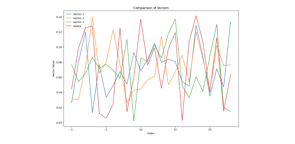 Comparison between query vector and top three most similar vectors
Conclusion
In this article, we’ve explored the combination of time series databases and vector databases, focusing on the use case in Internet of Things (IoT) applications. Time series databases, such as InfluxDB, are highly efficient at storing and querying chronological data, which is crucial for applications like weather forecasting, stock market analysis, and sensor monitoring. However, they face limitations when it comes to performing similarity searches.
To overcome this, we combined time series databases with vector databases like Milvus, which store data in vector form, enabling efficient similarity searches using techniques like cosine similarity or Euclidean distance. By combining the two databases, the strengths of both systems can be fully utilized. As you can see in the example above, time series data from sensors can be stored in InfluxDB, while vector data can be stored in Milvus. This integration allows for advanced use cases like anomaly detection in real-time traffic conditions.
The code related to Milvus presented in this article can be accessed via this Colab notebook.
You can also take a look at this article that explores preprocessing methods to transform time series data into an embedding suitable for forecasting tasks.
Keep Reading

Our Journey to 35K+ GitHub Stars: The Real Story of Building Milvus from Scratch
Join us in celebrating Milvus, the vector database that hit 35.5K stars on GitHub. Discover our story and how we’re making AI solutions easier for developers.

Legal Document Analysis: Harnessing Zilliz Cloud's Semantic Search and RAG for Legal Insights
Enhance legal document analysis with Zilliz Cloud’s Semantic Search and RAG. Improve accuracy, efficiency, and scalability for contracts, case law, and compliance.

OpenAI o1: What Developers Need to Know
In this article, we will talk about the o1 series from a developer's perspective, exploring how these models can be implemented for sophisticated use cases.
