


Getting Started with Audio Data: Processing Techniques and Key Challenges
Discover audio data, its characteristics, processing techniques, and key challenges. Learn how to tackle them effectively in AI applications.
Read the entire series
- Top 10 Most Used Embedding Models for Audio Data
- Unlocking Pre-trained Models: A Developer’s Guide to Audio AI Tasks
- Choosing the Right Audio Transformer: An In-depth Comparison
- From Text to Speech: A Deep Dive into TTS Technologies
- Getting Started with Audio Data: Processing Techniques and Key Challenges
- Enhancing Multimodal AI: Bridging Audio, Text, and Vector Search
- Scaling Audio Similarity Search with Vector Databases
The global speech and voice recognition market is booming. Experts have projected that the total will reach USD 17.33 billion in 2025 to USD 61.27 billion by 2033.
The numbers speak for themselves. Voice assistants process billions of queries daily, music platforms analyze songs for recommendations, and AI hearing aids enhance the sound in real time. Despite this growth, raw audio remains a complex challenge.
A study indicates that the Global AI Audio Processing Software Market size is expected to be worth around USD 18 Billion by 2033. Advancements in speech recognition and natural language processing technologies drive this growth. The volume of audio data is increasing rapidly, making efficient processing more challenging. To keep AI models reliable, we need better preprocessing and data-cleaning techniques.
This post, the first in A Developer’s Handbook to Mastering Audio AI, introduces developers to the fundamentals of audio data and essential preparation techniques. We break down core concepts and preprocessing methods to help you transform raw audio into clean, structured inputs for AI models. By the end, this post will equip you to process audio data and tackle key challenges in handling audio data using Python libraries.
Siri – Apple's Voice AI Assistant | Source
What is Audio Data?
Audio data is the digital representation of sound waves. It is captured by converting analog sound signals (like human speech, music, or environmental noise) into a series of numerical values. This process involves sampling the continuous sound wave at discrete intervals and storing it in formats computers can process. Common audio file formats include:
Waveform Audio File(WAV): Uncompressed, high-quality audio ideal for editing.
MPEG-1 Audio Layer 3(MP3): Compressed format that sacrifices some quality for smaller file sizes.
Free Lossless Audio Codec(FLAC): Lossless compression, preserving quality while reducing storage.
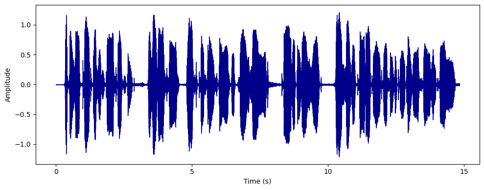
A Graphical Representation of Audio Data
Characteristics of Audio Data
Audio data has several key characteristics that impact its quality and usability in AI applications. These are defined below::
Sampling Rate: Sampling rate refers to the number of audio snapshots taken per second, measured in kilohertz (kHz). A higher sampling rate captures more detail but also increases file size. For example, AI speech recognition systems use a 16 kHz sampling rate to balance clarity and efficiency.
Bit Depth: Bit depth determines the precision of each audio sample, affecting dynamic resolution. Higher bit depths capture a wider range of sounds. For example, a 24-bit depth is used in AI-based music generation to capture nuanced sound variations.
Channels: Channels indicate the number of audio tracks, with mono (one channel) and stereo (two channels) being the most common. Stereo enhances spatial context for immersive experiences, while mono is ideal for voice clarity. For example, podcasts are typically mono, while music is often mixed in stereo to create space.
Dynamic Range: Dynamic range is the difference between the quietest and loudest sounds in an audio recording. A wide dynamic range requires careful normalization to prevent clipping or inaudible details. For example, the dynamic range in a classical music recording is the difference between a soft piano solo and a loud brass section.
Frequency: Frequency refers to the pitch of sound, measured in Hertz (Hz), with human hearing ranging from 20 Hz to 20 kHz. AI models often filter out irrelevant frequencies to enhance speech processing. For example, AI speech recognition models filter out frequencies below 300 Hz to focus on human speech.
These properties determine how accurately audio represents real-world sound and influence preprocessing steps like noise reduction or feature extraction.
Audio Preprocessing Techniques
Preprocessing is the crucial first step in AI-based audio analysis. It transforms raw, unstructured audio data into clean, usable, and standardized formats for analysis and model training. Preprocessing steps like data cleaning, resampling, normalization, and segmentation ensure the data is ready for reliable AI models.
In this guide, we'll use librosa, noisereduce, pydub, numpy, and matplotlib.pyplot, popular libraries for audio manipulation and data visualization, to demonstrate each preprocessing step. The built-in "trumpet" audio dataset from librosa will serve as our dataset for demonstration. Numpy will be used for numerical operations, while matplotlib.pyplot will help plot the graphs for visualizing the audio signals.
Data Cleaning
Data cleaning refers to removing unwanted noise and artifacts from raw audio, ensuring the sound quality is as high as possible. In this step, we focus on eliminating background noise, clicks, and distortions that can interfere with further analysis.
For example, if you’re working with a noisy audio clip, cleaning it will allow you to focus on the main audio features without distractions. We can use noise reduction techniques such as those available in the noisereduce library. By applying noise reduction, we improve the signal-to-noise ratio and enhance the clarity of the audio for tasks like speech recognition or music analysis.
Code example
    import librosa
    import noisereduce as nr
    import librosa.display
    import matplotlib.pyplot as plt

    audio_path = librosa.example('trumpet')
    y, sr = librosa.load(audio_path, sr=None)
    cleaned_audio = nr.reduce_noise(y=y, sr=sr)
    plt.figure(figsize=(10, 6))
    librosa.display.waveshow(cleaned_audio, sr=sr)
    plt.title("Cleaned Trumpet Audio Signal")
    plt.xlabel("Time (s)")
    plt.ylabel("Amplitude")
    plt.tight_layout()
    plt.show()
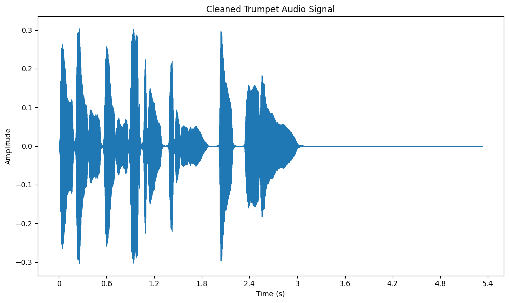
Audio Signals of Trumpet Dataset After Data Cleaning
Resampling
Resampling is the process of changing the sample rate of an audio signal to ensure consistency across different datasets. This is particularly important when working with audio from various sources that may have different sample rates.
For instance, if some audio clips are at 44.1 kHz and others at 22.05 kHz, resampling them to a common rate, such as 22.05 kHz, ensures uniformity across your dataset. In librosa, this is easily done using the librosa.resample function. Resampling guarantees that all audio files are processed in a consistent manner, which is crucial when performing tasks like feature extraction or classification.
Code example
    import librosa
    import librosa.display
    import matplotlib.pyplot as plt


    audio_path = librosa.example('trumpet')
    y, sr = librosa.load(audio_path, sr=None)
    target_sr = 16000
    y_resampled = librosa.resample(y, orig_sr=sr, target_sr=target_sr)
    plt.figure(figsize=(10, 6))
    librosa.display.waveshow(y_resampled, sr=target_sr)
    plt.title("Resampled Trumpet Audio Signal (16 kHz)")
    plt.xlabel("Time (s)")
    plt.ylabel("Amplitude")
    plt.tight_layout()
    plt.show()
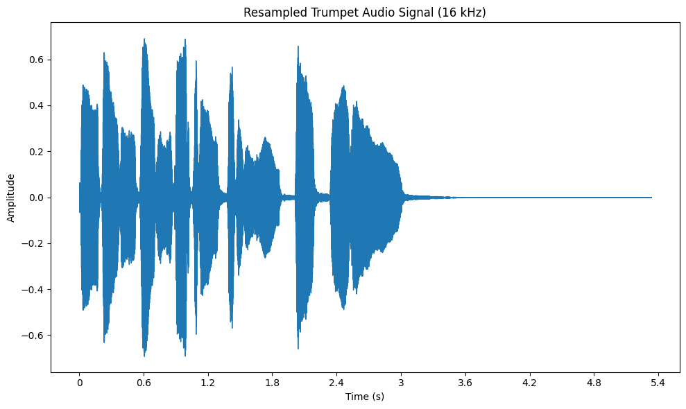
Audio Signals of the Trumpet Dataset After Resampling
Normalization
Normalization is a technique used to scale the amplitude of an audio signal to a standard range, typically between -1 and 1. This ensures that the audio is neither too loud (leading to clipping) nor too quiet. It’s an important step when dealing with audio from multiple sources that may have different volume levels.
Normalizing audio ensures consistent loudness across all clips, which is especially useful when creating playlists or preparing audio for machine learning models. In librosa, you can use the librosa.util.normalize function to normalize audio, and then visualize the waveform using matplotlib to see the effects of normalization.
Code example
    import librosa
    import librosa.display
    import matplotlib.pyplot as plt


    audio_path = librosa.example('trumpet')
    y, sr = librosa.load(audio_path, sr=None)
    y_normalized = librosa.util.normalize(y)
    plt.figure(figsize=(10, 6))
    librosa.display.waveshow(y_normalized, sr=sr)
    plt.title("Normalized Trumpet Audio Signal")
    plt.xlabel("Time (s)")
    plt.ylabel("Amplitude")
    plt.tight_layout()
    plt.show()
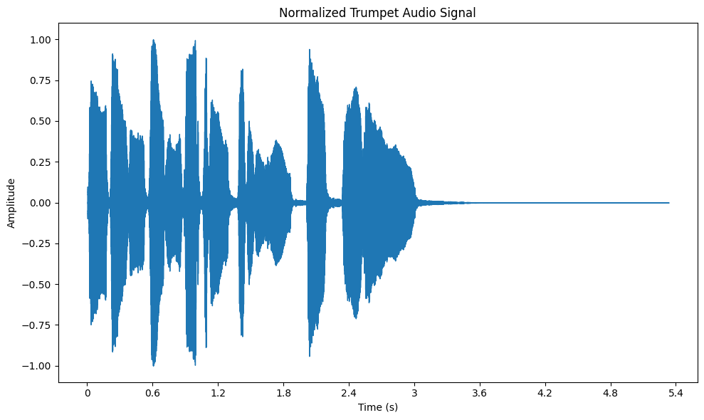
Audio Signals of the Trumpet Dataset After Normalization
Segmentation
Segmentation involves splitting an audio file into smaller, more manageable chunks. This is useful when dealing with long audio files that need to be analyzed in smaller sections. For example, if you're analyzing a long recording of a musical performance, you may want to segment the audio into individual notes or phrases.
Using segmentation, we can focus on specific parts of the audio without the need to process the entire file at once. This makes the analysis more efficient. The pydub library provides an easy way to segment audio. It allows us to break a file into specific durations, like 2-second chunks, for targeted analysis.
Code example
    from pydub import AudioSegment
    audio_path = librosa.example('trumpet')
    y, sr = librosa.load(audio_path, sr=None)
    audio_segment = AudioSegment(
        y.tobytes(),
        frame_rate=sr,
        sample_width=2,
        channels=1
    )
    segment_length = 10 * 1000
    segments = []
    for start_ms in range(0, len(audio_segment), segment_length):
        segment = audio_segment[start_ms:start_ms + segment_length]
        segments.append(segment)
    segments[0].export("segment_0.wav", format="wav")
    print("First segment saved as 'segment_0.wav'")
Feature Extraction Techniques
Feature extraction techniques convert raw audio into structured data, which helps machines process and analyze sound effectively. These techniques reveal patterns and features crucial for tasks like speech recognition and music analysis. Here are some key techniques:
Spectrograms and MFCCs
A Spectrogram visualizes how the frequencies in an audio signal change over time, combining time, frequency, and amplitude into a single graph. It is created using the Short-Time Fourier Transform (STFT), which splits the audio into small time segments and computes the frequency spectrum for each.
For example, in a music recording, a spectrogram can reveal the distinct frequencies of instruments like trumpets or violins, showing how they contribute to the overall sound. In speech processing, spectrograms help identify vowel sounds, as each vowel has a unique frequency signature.
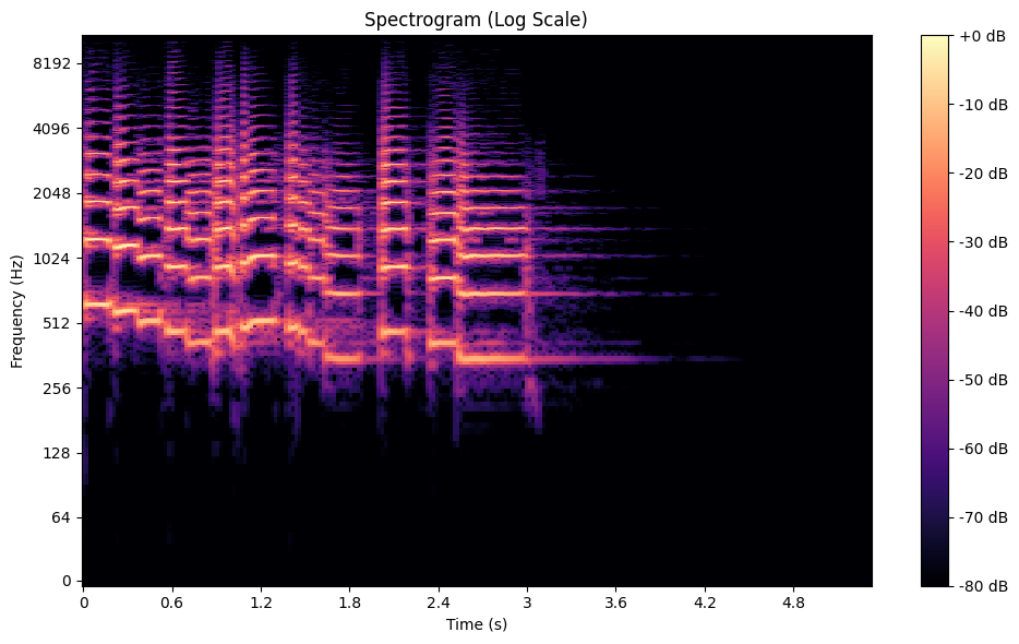
A Spectrogram of the Trumpet Dataset
A mel spectrogram is a variation that maps frequencies to the mel scale, which mimics the human ear’s sensitivity to sound. Unlike a linear frequency scale, the mel scale emphasizes lower frequencies, where humans are more perceptive. This makes mel spectrograms ideal for speech and music analysis. To create one, the STFT is applied, and the resulting spectra are passed through a mel filterbank.
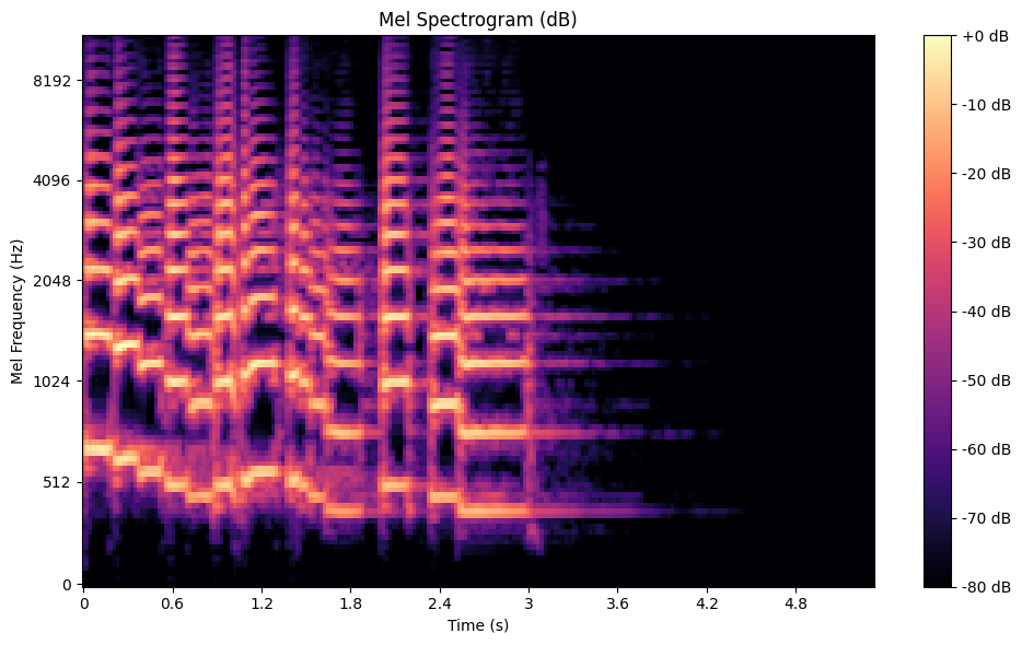
A Mel Spectrogram of the Trumpet Dataset
Mel-Frequency Cepstral Coefficients (MFCCs) take this a step further by compressing the mel spectrogram into a compact set of features. MFCCs are calculated by first pre-emphasizing the signal and splitting it into frames. Next, a Fast Fourier Transform (FFT) computes the power spectrum. The power spectrum is filtered through a mel-scale filter bank, logarithmically scaled, and finally transformed using a Discrete Cosine Transform (DCT). This process efficiently captures the essential timbral characteristics of the audio. Here’s how to generate MFCCs using Python:
    import librosa
    import librosa.display
    import matplotlib.pyplot as plt
    import numpy as np


    audio_path = librosa.example('trumpet')
    y, sr = librosa.load(audio_path, sr=None)
    mel_spectrogram = librosa.feature.melspectrogram(y=y, sr=sr, n_mels=128, fmax=8000)


    mel_spectrogram_db = librosa.power_to_db(mel_spectrogram, ref=np.max)
    plt.figure(figsize=(10, 6))
    librosa.display.specshow(mel_spectrogram_db, sr=sr, x_axis='time', y_axis='mel')
    plt.colorbar(format='%+2.0f dB')
    plt.title('Mel Spectrogram (dB)')
    plt.xlabel('Time (s)')
    plt.ylabel('Mel Frequency (Hz)')
    plt.tight_layout()
    plt.show()
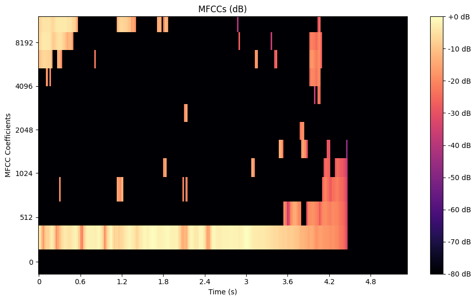
A Mel-Frequency Cepstral Coefficients of the Trumpet Dataset
Embeddings
Audio embeddings are high-level representations of audio data, often extracted using pre-trained deep learning models like Wav2Vec or VGGish. These embeddings capture semantic information, such as the emotional tone of speech or the genre of a song, making them ideal for transfer learning. For instance, a healthcare AI can use embeddings to classify cough sounds as indicative of specific diseases. Here’s how to extract embeddings using a pre-trained model:
    import torch
    from transformers import Wav2Vec2Processor, Wav2Vec2Model
    import librosa
    import matplotlib.pyplot as plt

    processor = Wav2Vec2Processor.from_pretrained("facebook/wav2vec2-large-960h")
    model = Wav2Vec2Model.from_pretrained("facebook/wav2vec2-large-960h")
    audio_path = librosa.example('trumpet')
    y, sr = librosa.load(audio_path, sr=16000)  # Ensure the sample rate is 16kHz, as required by Wav2Vec2
    inputs = processor(y, sampling_rate=sr, return_tensors="pt", padding=True)
    with torch.no_grad():
        embeddings = model(**inputs).last_hidden_state
    plt.figure(figsize=(10, 6))
    plt.imshow(embeddings[0].numpy()[:, :50], aspect='auto', cmap='viridis')
    plt.title('Wav2Vec2 Audio Embeddings')
    plt.xlabel('Frames')
    plt.ylabel('Embedding Dimensions')
    plt.colorbar()
    plt.tight_layout()
    plt.show()
    print("Embedding shape:", embeddings.shape)
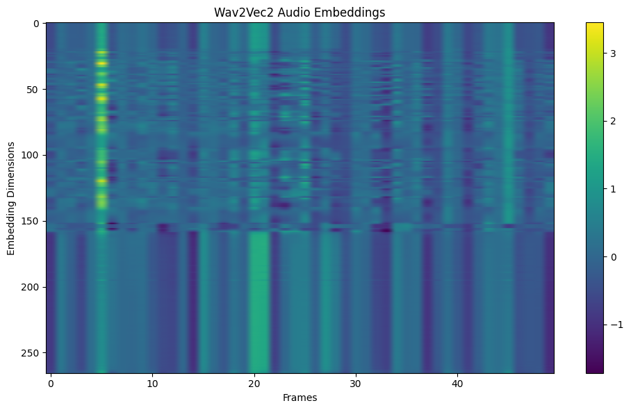
Visualization of Way2Vec2 Audio Embeddings Across Frames 0-40
Pitch and Tempo Analysis
Pitch refers to how high or low a sound is, essentially determining its musical note. In audio analysis, extracting pitch means identifying the fundamental frequency of the sound. One common method for this is the Short-Time Fourier Transform (STFT). With tools like Librosa, it's possible to track pitch values over time using functions like librosa.piptrack. This kind of analysis plays a key role in areas like music classification, where understanding tonal differences helps sort songs by genre or mood.
Recently, techniques like convolutional neural networks have been used to enhance the accuracy of pitch estimation, especially in more challenging audio environments.
Tempo indicates the speed of a piece of music, measured in beats per minute (BPM). Analyzing tempo involves detecting the timing of beats within an audio signal. Algorithms often identify peaks in energy or spectral changes to estimate tempo. Librosa provides the librosa.beat.beat_track function to estimate overall tempo and beat positions.
Tempo analysis is essential for tasks like DJ software or creating playlists, where it's important to match the pace of different tracks for a smooth experience. Recently, new methods have improved tempo estimation, even in challenging environments with noise or reverb.
Here’s how to analyze pitch and tempo using librosa:
    import librosa
    import librosa.display
    import matplotlib.pyplot as plt
    import numpy as np


    audio_path = librosa.example('trumpet')
    y, sr = librosa.load(audio_path, sr=None)
    pitches, magnitudes = librosa.piptrack(y=y, sr=sr)
    pitch_values = []
    for i in range(pitches.shape[1]):
        index = magnitudes[:, i].argmax()
        pitch = pitches[index, i]
        pitch_values.append(pitch if pitch > 0 else np.nan)


    tempo, beats = librosa.beat.beat_track(y=y, sr=sr)
    if isinstance(tempo, np.ndarray):
        tempo = tempo[0]


    plt.figure(figsize=(12, 6))
    plt.subplot(2, 1, 1)
    plt.plot(pitch_values, color='b')
    plt.title('Pitch Analysis')
    plt.xlabel('Frames')
    plt.ylabel('Pitch (Hz)')


    plt.subplot(2, 1, 2)
    librosa.display.waveshow(y, sr=sr, alpha=0.6)
    plt.vlines(librosa.frames_to_time(beats, sr=sr), -1, 1, color='r', linestyle='--', label='Beats')
    plt.title(f'Tempo Analysis (Tempo: {tempo:.2f} BPM)')
    plt.xlabel('Time (s)')
    plt.ylabel('Amplitude')


    plt.tight_layout()
    plt.show()


    print(f"Estimated Tempo: {tempo:.2f} BPM")
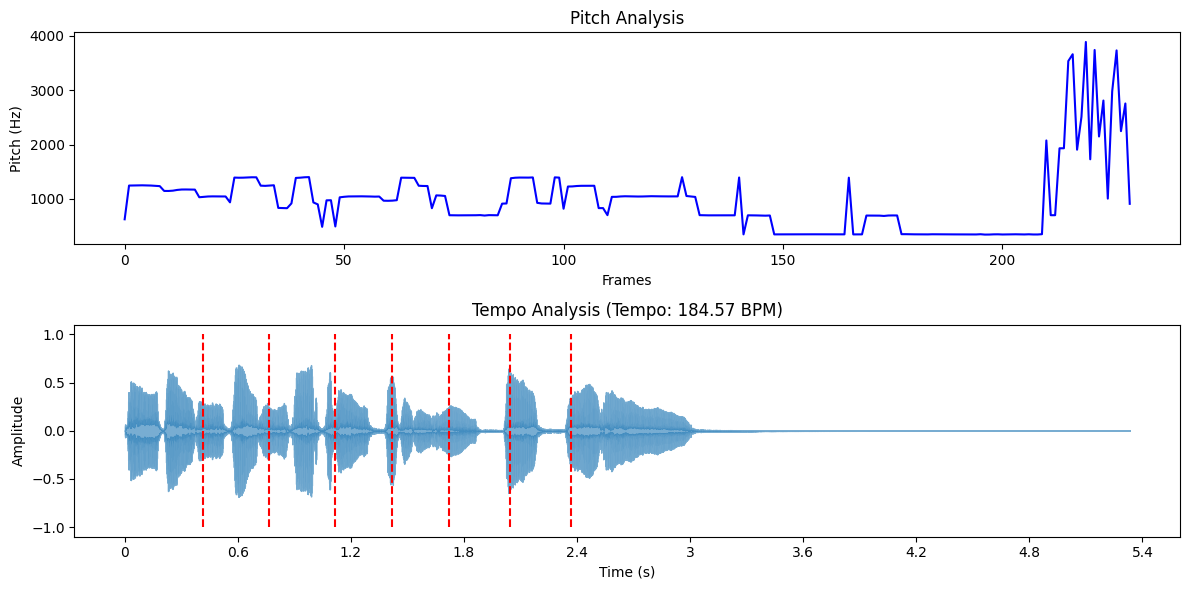
Pitch and Tempo Analysis of the Trumpet Dataset
Key Challenges in Working with Audio Data
While preprocessing and feature extraction form the backbone of audio AI workflows, real-world implementation faces persistent hurdles. These challenges test the limits of current tools and demand creative problem-solving. Here are a few key challenges:
Data Quality: Raw audio may have noise, distortions, or missing segments that degrade model performance. Techniques like noise reduction and normalization improve quality. High-quality labeled datasets are also crucial for training accurate models, requiring careful annotation and preprocessing.
Scalability: High-quality audio requires large storage and computational power. Efficient resampling, compression, and distributed computing help address this. Cloud-based storage and parallel processing frameworks can further optimize performance for large-scale applications.
Domain-Specific Requirements: Different applications have unique needs, making universal solutions difficult. Custom pipelines and expert knowledge are essential. For example, speech recognition in legal settings requires different processing techniques than music analysis.
Real-Time Processing: Many audio AI applications, such as virtual assistants and live transcription services, require real-time processing. This demands low-latency models, optimized algorithms, and efficient hardware acceleration to ensure seamless user experiences.
Tools and Libraries for Audio Data Processing
To address these challenges, developers rely on specialized tools designed for audio processing.
Python Libraries
Python offers a rich ecosystem of libraries for audio data processing, making it a go-to choice for developers.
- Librosa: Librosa is a versatile library for audio analysis. It provides tools for loading audio, extracting features like MFCCs and spectrograms, and performing tasks like tempo estimation and pitch detection. For example, Librosa can help a music streaming platform analyze song rhythms or classify genres.
- PyDub: Ideal for audio file manipulation, PyDub simplifies tasks like slicing, merging, and resampling. For instance, a security system analyzing long call recordings can use PyDub to split them into shorter segments for keyword detection.
- TorchAudio: Built for deep learning, TorchAudio integrates seamlessly with PyTorch, offering tools for loading audio, applying transformations, and extracting embeddings. It’s particularly useful for training custom audio AI models, such as speech-to-text systems.
Visualization Tools
Visualization tools help us better understand the audio data and its transformations. These tools are key for interpreting the results of preprocessing steps and for debugging.
- Matplotlib: A popular plotting library, Matplotlib can visualize waveforms, spectrograms, and MFCCs. Plotting a spectrogram, for example, helps identify frequency patterns in a music track or speech recording.
- Plotly: For interactive visualizations, Plotly allows users to zoom, pan, and explore audio data in detail. This is especially useful for analyzing complex audio signals, such as identifying anomalies in industrial machine sounds.
Summary
Audio AI’s rapid growth demands careful data preparation. Raw audio often contains noise and inconsistencies that hinder AI performance. Preprocessing addresses these issues through key steps: cleaning unwanted sounds, adjusting sample rates, balancing volume levels, and splitting files into manageable clips. These techniques create uniform, high-quality inputs for reliable analysis.
Effective processing unlocks audio’s potential. Features like spectral patterns and semantic embeddings help machines understand context and meaning. Challenges remain in scaling these methods and adapting them to specialized needs. By prioritizing clear preprocessing and modern tools, developers can build AI systems that transform real-world audio into actionable insights across healthcare, security, and entertainment. The future of sound-driven innovation starts with mastering these fundamentals.
Related Resources
 Haziqa Sajid
Digital Storytelling for Data, AI, B2B & SaaS
- What is Audio Data?
- Characteristics of Audio Data
- Audio Preprocessing Techniques
- Feature Extraction Techniques
- Key Challenges in Working with Audio Data
- Tools and Libraries for Audio Data Processing
- Summary
- Related Resources
Content
Start Free, Scale Easily
Try the fully-managed vector database built for your GenAI applications.
Try Zilliz Cloud for FreeKeep Reading
Top 10 Most Used Embedding Models for Audio Data
Explore the 10 most popular audio embedding models including Wav2Vec 2.0, VGGish, and OpenL3. Learn how they transform sound into vectors for AI applications
Choosing the Right Audio Transformer: An In-depth Comparison
Discover how audio transformers enhance sound processing. Explore their principles, selection criteria, popular models, applications, and key challenges.

Scaling Audio Similarity Search with Vector Databases
Discover how vector databases like Milvus and Zilliz Cloud enable efficient audio similarity search at scale, transforming music recommendations and audio retrieval applications.