Master Machine Learning: Batch Gradient Descent Explained

Master Machine Learning: Batch Gradient Descent Explained
Batch gradient descent is the gold standard of optimization in machine learning, known for its accuracy and stability. By calculating the gradients of the cost function over the whole dataset, it ensures consistent updates that lead to good model training. This post will go into how batch gradient descent works, its pros and cons and how it’s used in real world machine learning.
Summary
Gradient descent is the most basic optimization method in machine learning that minimizes loss by iteratively updating model parameters based on the cost function.
Batch gradient descent uses the whole training dataset for gradient calculations, it’s stable and consistent but requires a lot of computational resources.
Batch gradient descent can be improved by choosing the right batch size and practices to handle large datasets and monitor convergence.
Gradient Descent Basics
 An illustration depicting the fundamentals of gradient descent
At its heart gradient descent is a way to optimize model parameters to minimize loss in machine learning. This optimization process iteratively moves the parameters of a model in the opposite direction of the gradient of a loss function which measures the error between predicted and actual outcomes. The goal is to find the parameters that give the lowest error so the model performs well.
Gradient descent is used in many real world applications from deep learning to financial modeling. To understand its importance you need to know the basics that underlie this powerful optimization technique.
Cost Function
The cost function is a mathematical concept that measures how well a model does in making predictions. It measures the difference between predicted outcomes and actual outcomes and gives a measure of the model’s performance. Minimizing the cost function optimizes the model’s parameters and improves accuracy.
In practice the cost function guides the optimization process by telling the model how well its predictions match the actual outcomes. This allows us to compute the gradients which are then used to move the parameters in the direction that reduces the error. The key is to calculate and interpret the cost function correctly to steer the model towards better performance.
Learning Rate and Its Effects
The learning rate is a key hyperparameter in gradient descent that controls the amount of change to the model’s parameters during optimization. A good learning rate can make a big difference in the speed and stability of the training process. If the learning rate is too low the model will converge very slowly and training will be inefficient. If the learning rate is too high the model will overshoot the minimum and diverge.
Finding the right balance with the learning rate is key to training the model. A good learning rate allows the optimization to go steady, minimize the cost function without instability or slow convergence. This balance is important for optimal performance and efficiency.
Local Minima and Global Minima
In the loss function landscape local minima are points where the gradient is zero but not the lowest points overall. Local minima can trap the optimization and result in suboptimal model performance. Global minima is the absolute lowest point in the loss function landscape, the optimal solution for the model.
Local and global minima is a big challenge in gradient descent. Using different initial weights and momentum can help to avoid local minima and guide the optimization to the global minimum.
Knowing the difference between local and global minima is important to optimize machine learning models.
Batch Gradient Descent
 A visual representation of batch gradient descent in action
Batch gradient descent is the original gradient descent algorithm. Batch gradient descent looks at all the training data at once when adjusting the model. It's like considering every piece of evidence before making a decision. This method uses the entire dataset to calculate how to improve the model in each step, unlike other approaches that only use parts of the data at a time.This is thorough but can be slow for large datasets.
Batch gradient descent is good at converging to the optimal solution but that comes at the cost of computational resources. You need to balance computational efficiency and model accuracy to use batch gradient descent.
How Batch Gradient Descent Works
Batch gradient descent updates the model using all the training data at once. It's like baking a cake where you mix all ingredients together before putting it in the oven. This method calculates how to improve the model by looking at every single example in your dataset in one go, rather than piece by piece. This process the entire dataset before updating any of the model’s parameters so the gradient is calculated accurately. The computed gradients are then used to update the parameters moving them in the direction of the cost function.
This approach gives stable and predictable convergence but can be slow and resource intensive especially for large datasets. Since you need to process the entire dataset before updating anything, batch gradient descent can be slow.
Despite these challenges, its precision and stability make it a valuable tool in machine learning.
Batch Gradient Descent Advantages
One of the biggest advantages of batch gradient descent is that it converges to the optimal solution stably and consistently. Using the entire dataset gives you a stable error gradient which leads to predictable convergence. This is very useful for convex optimization problems where the error surface is smooth and the convergence is steady.
Batch gradient descent’s consistency on smooth error manifolds makes it a good method for optimizing machine learning models. The stable error gradient means the optimization process goes smoothly and reduces the chance of fluctuations and instability. This is very useful in many real world applications.
Batch Gradient Descent Drawbacks
Despite the advantages, batch gradient descent has big drawbacks, mainly its high computational cost. Processing the entire dataset before making any updates can be slow and resource hungry and not practical for very large datasets. This inefficiency can lead to longer training time and more computational resources.
The high computational cost of batch gradient descent limits its practicality in machine learning especially for large scale problems. While it gives stable and precise updates, the trade off in terms of computational efficiency can be a big hurdle. Managing these trade offs is key to using batch gradient descent in real world scenarios.
Gradient Descent Variants
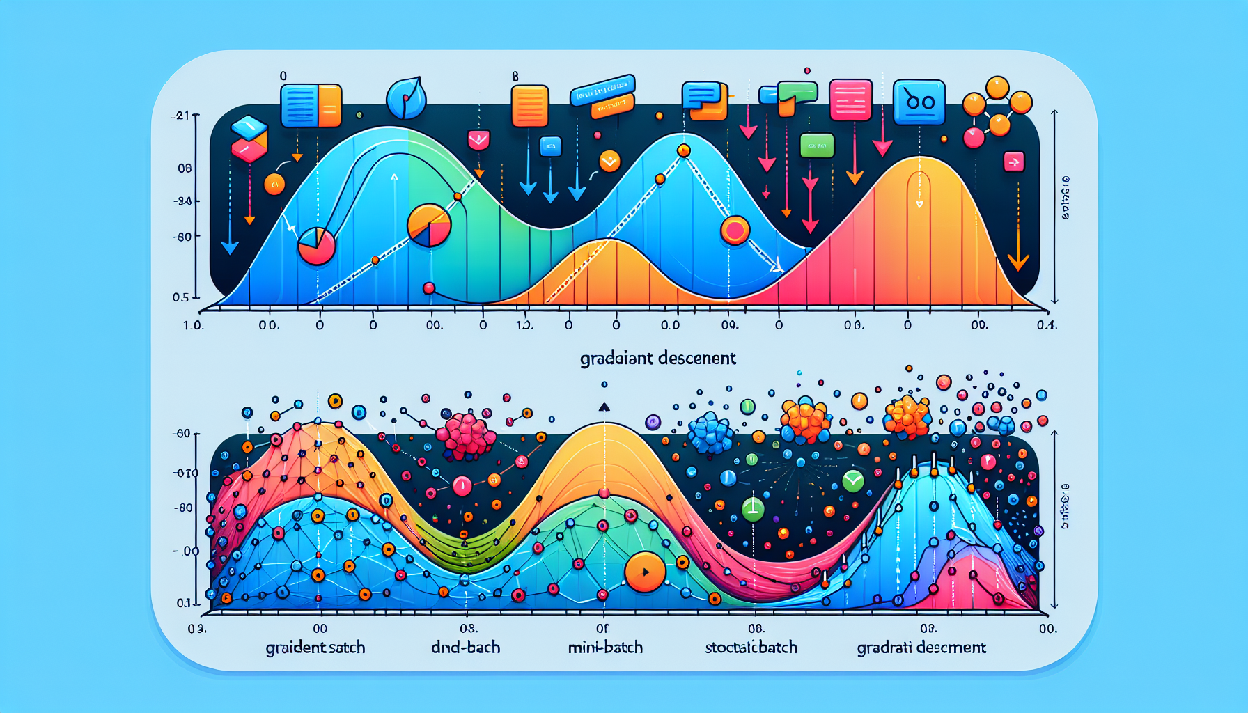
 An infographic comparing different gradient descent variants including stochastic and mini batch gradient descent
Choosing the right gradient descent for your machine learning models is crucial. Each variant has its pros and cons so it’s suitable for different scenarios and use cases.
This section compares batch gradient descent with stochastic gradient descent (SGD) and mini-batch gradient descent.
Stochastic Gradient Descent (SGD)
Stochastic Gradient Descent (SGD) is a stochastic approximation of the true cost gradient by updating the model weights after each sample is processed. Unlike batch gradient descent which processes the entire dataset, SGD updates once per sample so it’s faster but noisier during training.
The stochastic nature of SGD allows it to escape local minima better but the noise can make convergence less stable. This makes SGD suitable for large scale machine learning tasks where fast updates are important even if it means a trade-off in stability.
Mini Batch Gradient Descent
Mini batch gradient descent is a middle ground between batch and stochastic gradient descent. By using mini batches (a subset of the training samples), this method gets the best of both worlds. It uses vectorized operations so it’s faster with fewer iterations.
This gives us a way to handle cost functions with multiple local minima and a more balanced and efficient optimization. By reducing the batch size mini batch gradient descent can keep the gradient estimation accurate and fast. That’s why it’s used in many machine learning applications.
Batch Gradient Descent Practicalities
 An illustration focusing on practical considerations for batch gradient descent
Batch gradient descent has many practicalities to consider. From batch size to large datasets and convergence monitoring, these are key to performance and efficiency.
Batch Size
Choosing the right batch size is critical to balancing compute and model quality. In mini-batch gradient descent we typically choose batch sizes that are powers of 2, 32 or 64 for example.
This keeps compute efficient and training quality high.
Large Datasets
Handling large datasets is a big challenge in batch gradient descent due to the high memory and compute requirements. Data shuffling and parallel processing can help with these challenges, so batches are representative of the full dataset and improve the learning in batch gd.
These keep efficient and effective for large scale machine learning.
Convergence Monitoring
Monitoring the model convergence is key to training effectively and minimizing the loss. Visualization tools can help with this, to find the optimal stopping criteria and not to compute unnecessary once the model has converged enough.
This approach ensures an efficient and effective training process.
Common Issues and Solutions
 An illustration depicting common pitfalls in machine learning related to gradient descent
Gradient descent is a great optimization method but not without its pitfalls. Overfitting, underfitting and non-convex functions can kill your model performance.
This section covers the solutions to these problems so your models can perform optimally.
Overfitting and Underfitting
Overfitting happens when a model becomes too focused on the specific examples it was trained on. It's like memorizing answers instead of understanding the subject. This can make the model perform poorly on new, unseen data.
Underfitting occurs when a model is too basic to grasp the important patterns in the data. It's similar to using a straight line to describe a curved relationship. The model misses key trends, resulting in poor performance on both training and new data.
Using learning curves to visualize training and validation loss and cross-validation helps to identify and fix these issues so the model generalizes well to new data.
Learning Rates
Dynamic learning rates can prevent training from getting stuck and ensure progress during model optimization. Balancing learning rates with batch sizes optimizes model training and converges faster.
So training is effective and efficient.
Non-Convex Functions
Non-convex functions is a big challenge in optimization. Using techniques like random restarts can help to avoid local minima and navigate non-convex optimization problems.
These strategies are crucial for achieving optimal solutions in complex loss landscapes.
Real-World Applications
Batch gradient descent is used in many areas, computer vision, natural language processing, financial modeling etc. Here we will see two examples of it’s application in two prominent areas and see how versatile and effective it is.
Image Recognition
In image recognition tasks batch gradient descent is used to train deep learning models to classify images accurately. By optimizing convolutional neural networks it improves feature extraction and classification accuracy making it a powerful tool in computer vision.
Natural Language Processing
In natural language processing batch gradient descent is used in tasks like sentiment analysis and language translation to optimize model performance to predict linguistic patterns. It’s ability to handle large datasets makes it very useful in NLP models.
Summary
Batch gradient descent is key to optimising machine learning models. From the basics to practicalities and common gotchas, this has covered it all. Apply this and you’ll be able to improve your models’ performance and efficiency.
FAQs
What’s the main advantage of batch gradient descent over stochastic gradient descent?
The main advantage of batch gradient descent is that it converges more steadily to the optimal solution as it uses the entire dataset to compute the gradient, hence more precise updates and less fluctuation in the error gradient.
How does the learning rate affect gradient descent?
The learning rate is critical to gradient descent as it determines the size of the updates to the model parameters. An optimal learning rate gives efficient convergence and stability, a bad one gives slow convergence or divergence.
How to handle large datasets in batch gradient descent?
To handle large datasets in batch gradient descent, data shuffling and parallel processing is a must. These will ensure that the batches are a good representation of the entire dataset and hence the learning.
How to prevent overfitting in my machine learning model?
To prevent overfitting in your machine learning model, use learning curves to visualise training and validation loss and cross-validation to generalise to unseen data.
What is mini-batch gradient descent and how is it different from batch and stochastic gradient descent?
Mini-batch gradient descent is a balance between batch and stochastic gradient descent by processing subsets of the training data, hence faster convergence and stability. This is more computationally efficient and is used in many machine learning applications.
- Summary
- Gradient Descent Basics
- Batch Gradient Descent
- Gradient Descent Variants
- Batch Gradient Descent Practicalities
- Common Issues and Solutions
- Real-World Applications
- Summary
- FAQs
Content
Start Free, Scale Easily
Try the fully-managed vector database built for your GenAI applications.
Try Zilliz Cloud for Free