RAG Without OpenAI: BentoML, OctoAI and Milvus
This article was originally published in The New Stack and is reposted here with permission.
Expanded retrieval augmented generation options can eliminate developer dependence on OpenAI
ChatGPT brought AI to the forefront of public knowledge in 2023. However, there are now many more options, so we’re no longer tied to OpenAI. This is the third entry in a series of blogs on how you can build retrieval augmented generation (RAG) apps using LLMs that aren’t OpenAI’s GPT. Here’s where you can find part 1 and part 2. The GitHub repo for this project can be found here.
In this tutorial we will use BentoML to serve embeddings, OctoAI to get the LLM and Milvus as our vector database. We cover:
Serving embeddings with BentoML
Inserting your data into a vector database for RAG
Creating your Milvus collection
Parsing and embedding your data for insertion
Set Up your LLM for RAG
Giving the LLM instructions
A RAG example
Summary of the BOM dot COM: BentoML, OctoAI and Milvus for RAG
Serving Embeddings with BentoML
We can use sentence embeddings served through BentoML using its Sentence Transformers Embeddings repository. Let’s briefly cover what’s going on with this repo. The main thing to look at is the service.py file. Basically, it spins up a server and puts an API endpoint on it. Within the API endpoint, it is loading the all-MiniLM-L6-v2 from Hugging Face and using it to create embeddings.
That repository spins up a server and gives us an endpoint to hit at <http://localhost:3000>. To use this endpoint, we import bentoml and spin up an HTTP client using the SyncHTTPClient native object type.
import bentoml
bento_client = bentoml.SyncHTTPClient("http://localhost:3000")
Once we connect to the client, we create a function that gets a list of embeddings from a list of strings. One thing to note is that I split the lists into 25 strings at a time. This is mostly because we are using a synchronous endpoint. Splitting up the list of strings makes the calls less computationally expensive and avoids timeouts.
After splitting the list into 25 sections, we call the bento_client we created above to encode these sentences. The BentoML client returns a list of vectors, effectively a list of lists. We take each of these vectors and append them to our empty embedding list. At the end of this loop we return the final list of embeddings.
If there are not more than 25 strings in the list of texts, we simply call the encode method from the client on the passed in list of strings.
def get_embeddings(texts: list) -> list:
   if len(texts) > 25:
       splits = [texts[x:x+25] for x in range(0, len(texts), 25)]
       embeddings = []
       for split in splits:
           embedding_split = bento_client.encode(
               sentences = split
           )
           for embedding in embedding_split:
               embeddings.append(embedding)
       return embeddings
   return bento_client.encode(
       sentences=texts,
   )
Inserting Your Data into a Vector Database for RAG
With our embedding function prepared, we can prepare our data to insert into Milvus for our RAG application. The first step in this section is to start and connect to Milvus. There is a docker-compose.yml file located in the repository linked above. You can also find the Milvus Docker Compose on this docs page.
If you have Docker installed and downloaded that repo, you should be able to run docker compose up -d to spin up Milvus. Once your Milvus server is up, it’s time to connect to it. For this part, we simply import the connections module and call connect with the host (localhost or 127.0.0.1) and port (19530). The code block below also defines two constants - a collection name and the dimension. You can make up whatever collection name you want. The dimension size comes from the size of the embedding model, all-MiniLM-L6-v2.
from pymilvus import connections
COLLECTION_NAME = "bmo_test"
DIMENSION = 384
connections.connect(host="localhost", port=19530)
Creating Your Milvus Collection
Creating a collection in Milvus involves two steps: first, defining the schema, and second, defining the index. For this section, we need four modules: FieldSchema defines a field, CollectionSchema defines a collection, DataType tells us what type of data will be in a field and Collection is the object that Milvus uses to create collections.
We can define the entire schema for the collection here. Or, we can simply define the two necessary pieces: id and embedding. Then, when it comes time to define the schema, we pass a parameter, enabled_dynamic_field, that lets us insert whatever fields we want as long as we also have the id and embedding fields. This lets us treat inserting data into Milvus the same way we would treat a NoSQL database like MongoDB. Next, we simply create the collection with the previously given name and schema.
from pymilvus import FieldSchema, CollectionSchema, DataType, Collection
# id and embedding are required to define
fields = [
   FieldSchema(name="id", dtype=DataType.INT64, is_primary=True, auto_id=True),
   FieldSchema(name="embedding", dtype=DataType.FLOAT_VECTOR, dim=DIMENSION)
]
# "enable_dynamic_field" lets us insert data with any metadata fields
schema = CollectionSchema(fields=fields, enable_dynamic_field=True)
# define the collection name and pass the schema
collection = Collection(name=COLLECTION_NAME, schema=schema)
Now that we have created our collection, we need to define the index. In terms of search, an “index” defines how we are going to map our data out for retrieval. We use HSNW (hierarchical navigable small worlds) to index our data for this project. We also need to define how we’re going to measure vector distance. In this example, we use the inner product or IP.
Each of the 11 index types offered in Milvus has a different set of parameters. For HNSW, we have two parameters to tune: “M”, and “efConstruction”. “M” is the upper bound for the degree of a node in each graph, and “efConstruction” is the exploratory factor used during index construction.
From a practical standpoint, higher “M” and “efConstruction” both lead to better search. A higher “M” value means the index will take up more memory. A higher “efConstruction” value means it will take longer to build the index. You’ll have to play around with these to find the best values.
Once the index is defined, we create the index on a chosen field, in this case, embedding. Then we call load to load the collection into memory.
index_params = {
   "index_type": "HNSW", # one of 11 Milvus indexes
   "metric_type": "IP", # L2, Cosine, or IP
   "params": {
       "M": 8, # higher M = consumes more memory but better search quality
       "efConstruction": 64 # higher efConstruction = slower build, better search
   },
}
# pass the field to index on and the parameters to index with
collection.create_index(field_name="embedding", index_params=index_params)
# load the collection into memory
collection.load()
Parsing and Embedding Your Data for Insertion
With Milvus ready and the connection made, we can insert data into our vector database. But, we have to get the data ready to insert first. For this example, we have a bunch of txt files, available in the data folder of the repo. We split this data into chunks, embed it and store it in Milvus.
Let’s start by creating a function that chunks this text up. There are many ways to do chunking, but we’ll do this naively for this example. The function below takes a file, reads it in as a string and then splits it at every new line. It returns the newly created list of strings.
# naively chunk on newlines
def chunk_text(filename: str) -> list:
   with open(filename, "r") as f:
       text = f.read()
   sentences = text.split("n")
   return sentences
Next, we process each of the files we have. We get a list of all the file names and create an empty list to hold the chunked information. Then, we loop through all the files and run the above function on each to get a naive chunking of each file. Before we store the chunks, we need to clean them.
If you look at how an individual file is chunked, you'll see many empty lines, and we don't want empty lines. Some lines are just tabs or other special characters. To avoid those, we create an empty list and store only the chunks above a certain length. For simplicity, we can use seven characters.
Once we have a cleaned list of chunks from each document, we can store our data. We create a dictionary that maps each list of chunks to the document's name, in this case, the city name. Then, we append all of these to the empty list we made above.
import os
cities = os.listdir("data")
# store chunked text for each of the cities in a list of dicts
city_chunks = []
for city in cities:
   chunked = chunk_text(f"data/{city}")
   cleaned = []
   for chunk in chunked:
       if len(chunk) > 7:
           cleaned.append(chunk)
   mapped = {
       "city_name": city.split(".")[0],
       "chunks": cleaned
   }
   city_chunks.append(mapped)
With a set of chunked texts for each city ready to go, it’s time to get some embeddings. Milvus can take a list of dictionaries to insert into a collection so we can start with another empty list. For each of the dictionaries we created above, we need to get a list of embeddings to match the list of sentences.
We do this by directly calling the get_embeddings function we created in the section using BentoML on each of the list of chunks. Now, we need to match them up. Since the list embeddings and the list of sentences should match by index, we can enumerate through either list to match them up.
We match them up by creating a dictionary representing a single entry into Milvus. Each entry includes the embedding, the related sentence and the city. It’s optional to include the city, but let’s include it just so we can use it. Notice there’s no need to include an id in this entry. That’s because we chose to auto-increment the id when we made the schema above.
We add each of these entries to the list as we loop through them. At the end, we have a list of dictionaries with each dictionary representing a single-row entry to Milvus. We can then simply insert these entries into our Milvus collection. The last step here is to flush the entries so we can begin indexing them.
entries = []
for city_dict in city_chunks:
   embedding_list = get_embeddings(city_dict["chunks"]) # returns a list of lists
   # now match texts with embeddings and city name
   for i, embedding in enumerate(embedding_list):
       entry = {"embedding": embedding,
                "sentence": city_dict["chunks"][i], # poorly named cuz it's really a bunch of sentences, but meh
                "city": city_dict["city_name"]}
       entries.append(entry)
collection.insert(entries)
collection.flush()
Set Up Your LLM for RAG
Now, let’s get our LLM and get ready to rumble. And by rumble, I mean do some RAG. To do this section exactly as if, you need an account from OctoAI. You can also choose to drop in any LLM of your choice as a replacement.
In this first block of code, we simply load our environment variables, extract our OctoAI API token and spin up their client.
from dotenv import load_dotenv
load_dotenv()
os.environ["OCTOAI_TOKEN"] = os.getenv("OCTOAI_API_TOKEN")
from octoai.client import Client
octo_client = Client()
Giving the LLM Instructions
There are two things the LLM needs to know to do RAG: the question and the context. We can pass both of these at once by creating a function that takes two strings: the question and the context. Using this function, we use the OctoAI client’s chat completion to call an LLM. For this example, we use the Nous Research fine-tuned Mixtral model.
We give this model two “messages” that indicate how it should behave. First, we give a message to the LLM to tell it that it is answering a question from the user based solely on the given context. Next, we tell it that there will be a user, and we simply pass in the question.
The other parameters are for tuning the model behavior. We can control the maximum number of tokens and how “creative” the model acts.
The function then returns the output from the client in a JSON format.
def dorag(question: str, context: str):
   completion = octo_client.chat.completions.create(
   messages=[
           {
               "role": "system",
               "content": f"You are a helpful assistant. The user has a question. Answer the user question based only on the context: {context}"
           },
           {
               "role": "user",
               "content": f"{question}"
           }
       ],
       model="nous-hermes-2-mixtral-8x7b-dpo",
       max_tokens=512,
       presence_penalty=0,
       temperature=0.1,
       top_p=0.9,
   )
   return completion.model_dump()
A RAG Example
Now we’re ready. It’s time to ask a question. We can probably do this without creating a function, but making a function makes it nice and repeatable. This function simply intakes a question and then does RAG to answer it.
We start by embedding the question using the same embedding model we used to embed the documents. Next, we execute a search on Milvus. Notice that we pass the question into the get_embeddings function in list format, and then pass the outputted list directly into the data section of our Milvus search. This is just because of the way that the function signatures are set up, it’s easier to reuse them than rewrite multiple functions.
Inside our search call, we also need to provide a few more parameters. anns_field tells Milvus which field to do an approximate nearest neighbor search (ANNS) on. We also need to pass some parameters for the index. Make sure the metric type matches the one we used to make the index, in this case IP. We also have to use a matching index parameter, in this case ef, or exploratory factor.
A higher ef means longer search time, but higher recall. You can experiment with this, ef can go up to 2048; we’re using 16 for speed and simplicity. There are only thousands of entries in this dataset. Next, we also pass a limit parameter which tells us how many results to get back from Milvus, for this example, we can just go with five.
The last search parameter defines which fields we want back from our search. For this example, we can just get the sentence, which is the field we used to store our chunk of text. Once we have our search results back, we need to process them. Milvus returns an entity with hits in it, so we just grab the “sentence” from all five hits and join them with a period so it forms a list paragraph.
Then, we pass the question the user asked along with that paragraph into the dorag function we created above and just return the response.
def ask_a_question(question):
   embeddings = get_embeddings([question])
   res = collection.search(
       data=embeddings,  # search for the one (1) embedding returned as a list of lists
       anns_field="embedding",  # Search across embeddings
       param={"metric_type": "IP",
               "params": {"ef": 16}},
       limit = 5,  # get me the top 5 results
       output_fields=["sentence"]  # get the sentence/chunk and city
   )
   sentences = []
   for hits in res:
       for hit in hits:
           sentences.append(hit.entity.get("sentence"))
   context = ". ".join(sentences)
   return dorag(question, context)
print(ask_a_question("What state is Cambridge in?")["choices"][0]["message"]["content"])
For the example question asking which state Cambridge is in, we can just print the entire response from OctoAI. However, if we take the time to parse through it, it just looks nicer, and it should tell us that Cambridge is located in Massachusetts.

Summary of the BOM dot COM: BentoML, OctoAI, and Milvus for RAG
This example covered how you can do RAG without OpenAI or a framework. Notice that unlike some of our examples before, we also did not use LangChain or LlamaIndex. This time our stack was the BOM.COM — BentoML, OctoAI, and Milvus. We used BentoML’s serving capabilities to serve an embedding model endpoint, OctoAI’s LLM endpoints to access an open source model and Milvus as our vector database.
There are many ways to structure the order in which we use these different puzzle pieces. For this example, we started by spinning up a local server with BentoML to host an embedding model from Hugging Face. Next, we spun up a local Milvus instance using Docker Compose.
We used a simple method to chunk up our data, which was scraped from Wikipedia. Then, we took those chunks and passed them to our embedding model, hosted on BentoML, to get the vector embeddings to put into Milvus. With all of the vector embeddings in Milvus, we were fully set to do RAG.
The LLM we chose this time was the Nous Hermes fine-tuned Mixtral model, one of many open source models available on OctoAI. We created two functions to enable RAG. One function that passed in the question and context to the LLM, dorag, and another function that embedded the user question, searched Milvus, and then passed in the search results along with the question to the original RAG function. At the end, we tested our RAG with a simple question as a sanity check.
Keep Reading

Why I’m Against Claude Code’s Grep-Only Retrieval? It Just Burns Too Many Tokens
Learn how vector-based code retrieval cuts Claude Code token consumption by 40%. Open-source solution with easy MCP integration. Try claude-context today.

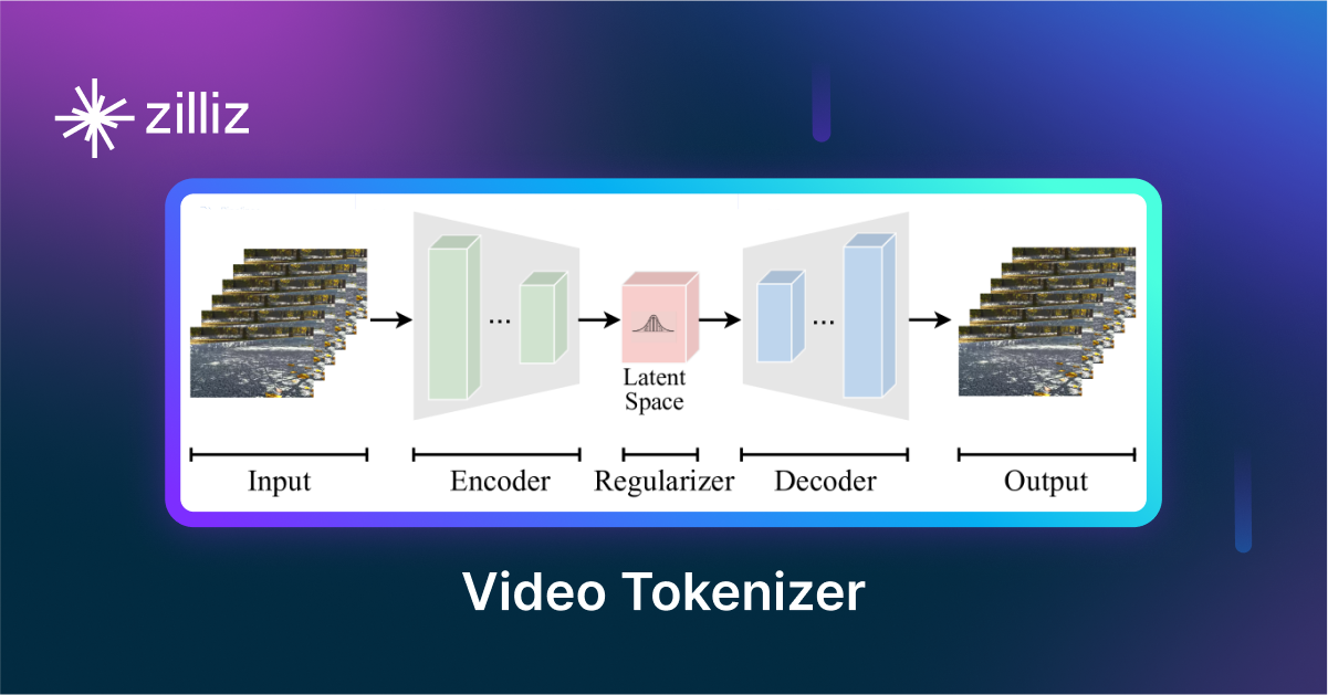
VidTok: Rethinking Video Processing with Compact Tokenization
VidTok tokenizes videos to reduce redundancy while preserving spatial and temporal details for efficient processing.

Vector Databases vs. Time Series Databases
Use a vector database for similarity search and semantic relationships; use a time series database for tracking value changes over time.
