AutoRegressive Integrated Moving Average (ARIMA)

AutoRegressive Integrated Moving Average (ARIMA)
Have you ever wondered how businesses accurately predict product demand for upcoming seasons and optimize their launches? That's where ARIMA comes into play. ARIMA is a statistical model that forecasts future time series values by analyzing past patterns.
Let's discuss ARIMA's importance, benefits, and challenges by going over how it works.
What is ARIMA?
AutoRegressive Integrated Moving Average (ARIMA) is a popular statistical model for time series forecasting. It uses historical data to understand dataset patterns and forecast future values. The model uses three components to predict future values: Auto-regression (AR), Differentiation (I), and Moving Average (MA). Each component shapes the model’s predictions by outlining a relationship between the past and future values.
Here’s what each component does:
Auto-regression (p): AR assumes that the future value depends on the past value. The AR order refers to the number of past values the model uses to predict the current value. For example, if the AR order is 3, the model predicts the current value based on the three most recent past values.
Differencing/ Integration (d): This determines the degree of differencing required to make a time series stationary. In non-stationary time series, where statistical properties like mean and variance change over time, applying differencing helps stabilize the series.
Moving Average (q): MA captures the relationship between the current value of a time series and past forecast errors. The MA order reflects the relationship between the current value of the time series and the past forecast errors. For example, MA(2) or MA of order 2 calculates the weighted average of the past two errors to predict the current value.
Mathematically, the ARIMA model is represented as ARIMA (p, d, q) and expressed as:
y′t=I+α1y′t−1+α2y′t−2+⋯+αpy′t−p+et+θ1et−1+θ2et−2+⋯+θqet−q
Where:
Yt: The current value of the time series
c: Constant term
φ₁, φ₂, ..., φp: Autoregressive coefficients
θ₁, θ₂, ..., θq: Moving average coefficients
εt: Noise error term
p: The order of the autoregression
q: The order of the moving average
d: The order of differencing/ integration
This represents that the current value of the differenced time series (y′t) is a linear combination of its past values (y′t-₁, y′t-₂, ..., y′t-p) and past error terms (et-₁, et-₂, ..., et-q).
How Does ARIMA Work?
Autocorrelation and moving averages are essential components of ARIMA models. Autocorrelation helps identify the direct relationships between past and current values while moving averages help account for the indirect effects of past forecast errors.
Here's a step-by-step breakdown of how they work together:
Stationarity
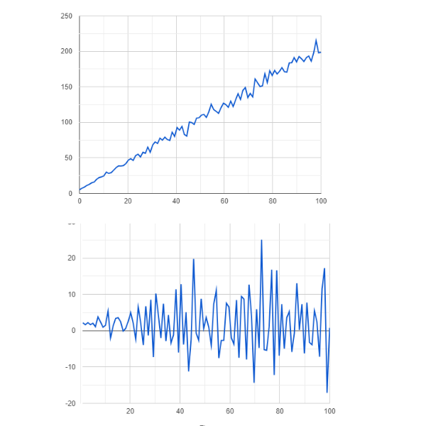
The first step in time series forecasting with ARIMA models is to ensure that the time series is stationary. Since non-stationary data can lead to inaccurate forecasts and biased model results, ARIMA is based on the assumption of stationarity. If the time series data is non-stationary, ARIMA applies differencing to make it stationary. This involves subtracting the previous value from the current value. The order of differencing (d) determines the number of times this process is repeated.
 Figure- Non-stationary vs stationary data .png
Figure: Non-stationary vs stationary data
Model Identification
Model identification determines the appropriate values for the autoregressive (p) and moving average (q) components. The autocorrelation function (ACF) and partial autocorrelation function (PACF) are essential tools for this process:
Autocorrelation Function
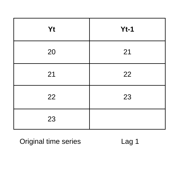
The autocorrelation function identifies the order of the autoregressive (AR) component (p). If it shows a correlation at lag k, it suggests that the current value is related to the value k periods ago, where k represents the number of lags (time steps) between the current value and a previous value in the time series.
Partial Autocorrelation Function
Partial autocorrelation function (PACF) identifies the order of the moving average (MA) component (q). If it shows a significant correlation at lag k, it indicates that the current value is related to the forecast error that occurred k periods ago.
 Figure- Lag-1 autocorrelation.png
Figure: Lag-1 autocorrelation
Model Estimation
After determining the autoregressive (AR) orders and moving average (MA) components, ARIMA estimates model parameters. Model parameters quantify the strength of the relationships between the current value and its past values (AR) and between the current value and past errors (MA).
Maximum likelihood estimation (MLE) is the most common method for parameter estimation in ARIMA models. MLE estimates model parameters by finding the values that maximize the likelihood of observing the given data. For ARIMA models, the likelihood function is typically based on the assumption that the errors are normally distributed. Least squares and Bayesian methods are other approaches for parameter estimation in ARIMA models.
Model Forecasting
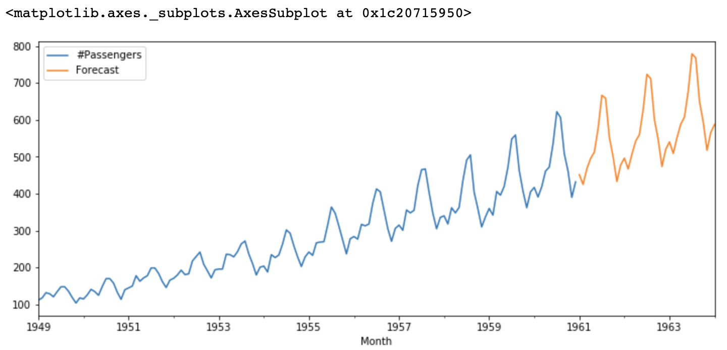
The estimated ARIMA model finally predicts future values based on historical data. If necessary, the model can also be refined by adjusting the orders of the AR and MA components or considering other factors like seasonality.
 Figure- ARIMA forecasts.png
Figure: ARIMA forecasts
Comparison with Similar Concepts
ARIMA is often compared to other similar concepts in the context of data analysis and forecasting. Here's a comparison to dismantle common misunderstandings:
ARIMA vs. SARIMA: SARIMA (Seasonal ARIMA) is an extension of ARIMA that specifically incorporates seasonality in time series data analysis. ARIMA is a statistical model for time series data without a clear seasonal pattern.
ARIMA vs. Exponential Smoothing: ARIMA and exponential smoothing are methods for time series forecasting. ARIMA uses statistical techniques to model the underlying patterns, including trends, seasonality, and autocorrelation. Exponential smoothing, on the other hand, applies a simpler method of weighted averaging, where recent observations are given more weight than older ones. While ARIMA is better suited for data with intricate patterns, exponential smoothing works well for time series with a relatively stable trend and minimal seasonality, making it less adaptable to complex data.
ARIMA vs. Vector Autoregression (VAR): VAR is suitable for multivariate time series forecasting where several variables influence each other. ARIMA is suitable for univariate time series and requires differencing the series to achieve stationarity.
Benefits and Challenges of ARIMA
ARIMA offers several benefits, making it one of the most widely used time series forecasting models. However, it also comes with certain challenges, which require considering your analysis's properties and specific goals before applying ARIMA.
Benefits
The benefits of using ARIMA models for time series forecasting include:
Flexibility: ARIMA can handle a wide range of time series data, including linear and non-linear trends, seasonal patterns, volatility, and autocorrelation. This allows it to address common characteristics of real-world time series, such as economic indicators and non-linear patterns in stock prices.
Simplicity: ARIMA models are easy to understand due to their simple functioning and transparent assumptions. They can handle long time series with a relatively large number of observations.
Accuracy: The accuracy of ARIMA models depends on the data quality. Therefore, considering assumptions and choosing appropriate models lead to accurate results.
Interpretability: ARIMA model parameters have clear interpretations, including autoregressive and moving average coefficients. These coefficients give insight into how past values and errors affect future values.
Wide Applicability: ARIMA models are widely used across industries for forecasting applications like financial modeling, demand forecasting, and load forecasting. Therefore, they are built into many programming languages and have a wide community of supporters.
Foundation for Other Models: ARIMA models are a foundation for more complex time series models such as SARIMA and ARIMAX. By accounting for additional factors, they help improve the accuracy of forecasts beyond the historical values of the time series.
Challenges
The challenges of ARIMA models include:
Stationarity Assumption: The ****ARIMA model assumes that the time series is stationary; if not, it transforms the data to achieve stationarity. However, many real-world datasets are non-stationary, and preprocessing them can complicate the modeling process.
Linear Relationships: ARIMA is a linear model and cannot capture complex non-linear relationships in the data. Therefore, it might not accurately capture sudden shifts in the data caused by economic crises, external shocks, etc.
Model Identification: The performance of the ARIMA model depends on selecting the appropriate parameters (p, d, q). However, it often requires trial and error or grid search methods and can lead to overfitting or underfitting.
Sensitivity to Outliers: ARIMA models can be sensitive to outliers, which can impact their performance. Therefore, careful data preprocessing is required to achieve the desired outcomes.
Long-term Forecasting: ARIMA isn’t well-suited for long-term forecasting. This is because ARIMA models are based on past patterns and may not adequately capture unforeseen events or structural changes in the data-generating process.
Use Cases, Tools, and Providers of ARIMA
ARIMA models are widely applied for time series forecasting and analysis in various fields. This includes economics and finance, demand forecasting, production and capacity planning, healthcare, etc.
For example, ARIMA models were used to forecast the spread of COVID-19 cases in India. The researchers trained the ARIMA models using daily COVID-19 case data from March 14 to May 3, 2020, which yielded satisfactory accuracy.
Many programming languages and statistical packages provide tools for implementing ARIMA models. They include:
R
R has extensive time series analysis capabilities, including ARIMA modeling. Multiple libraries, including stats, forecast, and tseries offer functions to implement the ARIMA model in R.
Python
Python also offers extensive statistical libraries to implement ARIMA. Some of these include Statsmodels, Numpy, and Pandas.
MATLAB
MATLAB is a commercial mathematical computing software with built-in functions for ARIMA modeling. It also allows integration with other software tools and programming languages to combine ARIMA modeling with other workflows.
FAQs of ARIMA
What is ARIMA used for?
AutoRegressive Integrated Moving Average (ARIMA) is a statistical model used for time series analysis and forecasting. It's a popular method for predicting future values of a time series based on its past values.
How does ARIMA differ from other time series forecasting models?
ARIMA differs from other time series forecasting models due to its flexibility, interpretability, and wide applicability. ARIMA can capture a wide range of patterns in time series data, including trends, seasonality, and autocorrelation. The parameters in an ARIMA model have clear interpretations, and they can serve as a baseline for comparison with more complex models.
How to interpret ARIMA forecasts?
ARIMA forecasts are typically interpreted as point estimates of the expected future values of the time series. Various metrics, such as mean squared error (MSE), mean absolute error (MAE), and root mean squared error (RMSE), can be used to evaluate forecast accuracy.
What are the assumptions of the ARIMA model?
Below are the assumptions of the ARIMA model:
Stationarity: The statistical properties of time series (mean, variance, autocorrelation) must remain constant over time.
Linearity: ARIMA assumes a linear relationship between the current value and its past values and errors.
Normality: The errors are assumed to be normally distributed.
No Autocorrelation in Errors: The errors are assumed to be uncorrelated.
Related Resources
Read more about storing and preprocessing time series data:
- What is ARIMA?
- How Does ARIMA Work?
- Comparison with Similar Concepts
- Benefits and Challenges of ARIMA
- Use Cases, Tools, and Providers of ARIMA
- FAQs of ARIMA
- Related Resources
Content
Start Free, Scale Easily
Try the fully-managed vector database built for your GenAI applications.
Try Zilliz Cloud for Free