



Milvus 3.0 vs Elasticsearch: Closing the Search Gap
Modern search needs two things at once: exact keyword matching and semantic similarity. Getting both usually means two systems, and paying for it in sync, cost, and complexity.
I worked at Elasticsearch for four years; I now do vector search at Zilliz. Rather than assert that one engine can cover both, I built something you can check: Milvus 3.0 and Elasticsearch 9 in two Docker containers on one machine: the same CPU and memory caps, the same Parquet file, the same vectors, the same analyzer chain; with every query running live, side by side. The repo is linked at the end so you can validate and run it on your own data.
TL; DR: for most teams, Milvus 3.0 covers both keyword and vector search well enough to replace the two-engine setup. A few capabilities are on the roadmap, and I flag those as they come up.
The search gap
Keyword search and vector search grew up in different engines, so covering both has meant compromising.
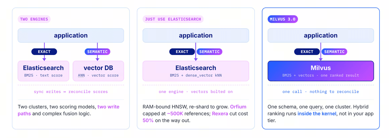
The usual compromise is two engines — Elasticsearch or OpenSearch for BM25, a vector database beside it for ANN. That's two clusters, two write paths, and two scoring models you reconcile yourself at query time.
The other is to use the keyword engine's own vector search and skip the second cluster. It works at small scale, but vectors are a Lucene plugin there: one HNSW graph per segment, RAM-bound, re-sharded to grow. There is a ceiling: Orfium, a global leader doing music rights management, is capped around 500K reference tracks before moving off.
Milvus 3.0 is one engine built for both: BM25 and vectors in one schema, a hybrid query as a single call with nothing to reconcile, and ranking in the kernel rather than your app tier (including reciprocal rank fusion - RRF - out of the box).
The rest of this post tests Milvus 3.0 against Elasticsearch, feature by feature, including where Milvus falls short. (OpenSearch shares the same Lucene vector architecture, so these points generally apply there too. The one Elasticsearch-specific difference is licensing: its RRF hybrid fusion is not an open source feature, flagged below.)
Who needs both exact and semantic search?
A single query often carries an exact constraint and a fuzzy intent at once, which is why AI applications hit this constantly:
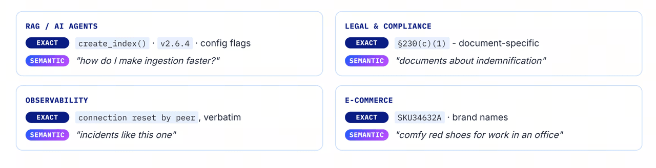
RAG and AI agents. Exact: a function name or version flag (
create_index(),v2.6.4). Semantic: "how do I make ingestion faster?"Legal and compliance. Exact: a clause or citation (
§230(c)(1)). Semantic: "documents about indemnification."Observability. Exact: an error string, verbatim (
connection reset by peer). Semantic: "incidents like this one."E-commerce. Exact: a SKU or brand. Semantic: "comfy red shoes for the office."
A keyword-only engine misses the intent; a vector-only engine misses the exact match. One engine has to do both.
Elasticsearch vs Milvus test setup: engines, data, and resource usage
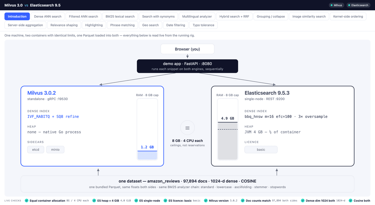
Both engines run as equals, so any difference is the engine, not the harness:
Engines: Milvus 3.0 standalone and Elasticsearch 9.5, each in Docker, each capped at 8 GB RAM / 4 CPUs (Milvus's
etcdand MinIO sidecars share that budget).Data: ~98K Amazon product records from one Parquet file, loaded byte-for-byte into both.
Vectors: the same 1024-d cosine floats on both sides. Generated once, loaded into each, so nothing is re-embedded.
Indexes: the same BM25 analyzer chain (standard tokenizer, lowercase, ASCII-folding, English stem/stop); Milvus uses RaBitQ 1-bit + SQ8 refinement for vectors, Elasticsearch uses
bbq_hnsw.Ground truth: recall is scored against exact brute-force neighbors over the full set, so the numbers are measured, not self-reported.
The demo's first tab verifies all of this live before any query runs.
Resource usage. For the same dataset, Milvus and its sidecars used about 0.5 GB of total memory, while the Elasticsearch footprint was around 5 GB.
Note: This isn't a benchmark: latency is shaped by JVM warm-up, container limits, and cold cache, so treat timings as directional and use published large-scale benchmarks for real numbers. Two more caveats carry through the rest: analyzer parity is close but not exact (the english stemmer is Porter1 on Elasticsearch, Porter2 on Milvus), and one hybrid path is licence-gated on Elasticsearch. What does reproduce on any box is feature coverage, query behavior, cross-engine agreement, and recall.
Below are results.
Dense (ANN) vector search: where recall comes from
# Milvus
client.search(
  "amazon_reviews",
  data=[qv],
  anns_field="text_vec",
  search_params={
    "params": {
      "nprobe": 4,
      "rbq_bits_query": 4,
      "refine_k": 2.0,
    },
  },
  limit=10,
)
# Elasticsearch
client.search(
  index="amazon_reviews",
  knn={
    "field": "text_vec",
    "query_vector": qv,
    "k": 100,
    "num_candidates": 100,
  },
  size=10,
)
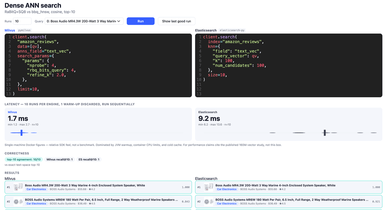
Both return essentially the same neighbors at high recall. The useful question is which knob buys it, because it isn't the obvious one. At the default (nprobe=64, refine_k=2.0) recall@10 is about 0.99; splitting the knobs apart:
nprobe | refine_k | recall@10 |
|---|---|---|
| unset | 1.0 | 0.928 |
| 64 | 1.0 | 0.930 |
| unset | 2.0 | 0.980 |
| 64 | 2.0 | 0.990 |
nprobe barely moves the number and saturates by about 8; raising refine_k from 1.0 to 2.0 is worth +0.05 to +0.06. Recall comes from the SQ8 pass rescoring the 1-bit candidates, not from scanning more of the graph. So if recall is low, raise refine_k, it's nearly free here. The trade: 1-bit quantization is lossy, and the refinement pass is what keeps recall high and memory low at once.
Full-text (BM25) search: parity on a smaller index
# Milvus
client.search(
  "amazon_reviews",
  data=["wireless earbuds"],
  anns_field="text_sparse",
  limit=10,
)
# Elasticsearch
client.search(
  index="amazon_reviews",
  query={"match": {"text_snippet": "wireless earbuds"}},
  size=10,
)
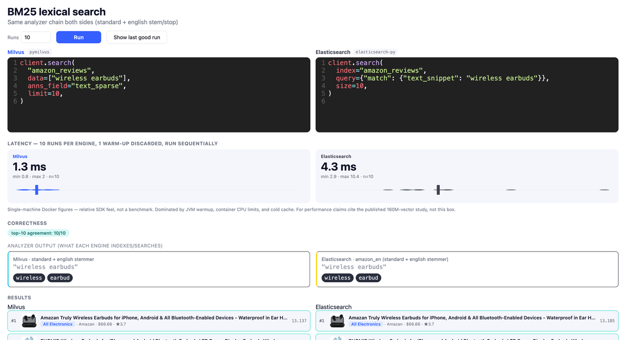
Same top-10, full agreement on the result set, and Milvus a little faster as often as not. The difference is underneath: Milvus's BM25 index — built for Zilliz Cloud, then contributed back to open source — runs about 3× smaller than Elasticsearch's, with no JVM heap behind it and no replica needed for durability.
Hybrid search: dense + BM25 with RRF
Hybrid search has to fuse dense and lexical results into one ranking. In Milvus, both requests go in together with a fusion ranker, in one call:
# Milvus
dense = AnnSearchRequest(
  [qv], "text_vec", SEARCH, limit=50)

sparse = AnnSearchRequest(
  ["wireless earbuds"], "text_sparse", {}, limit=50)

client.hybrid_search(
  "amazon_reviews",
  [dense, sparse],
  ranker=RRFRanker(),
  output_fields=["parent_asin"],
  limit=10,
)
The Elasticsearch version looks almost identical — two retrievers fused with rrf:
# Elasticsearch
sparse = {"standard": {"query": {
  "match": {"text_snippet": "wireless earbuds"}}}}

dense = {"knn": {
  "field": "text_vec", "query_vector": qv,
  "k": 50, "num_candidates": 100}}

client.search(
  index="amazon_reviews",
  retriever={"rrf": {
    "retrievers": [sparse, dense],
    "rank_window_size": 50,
  }},
  size=10,
)
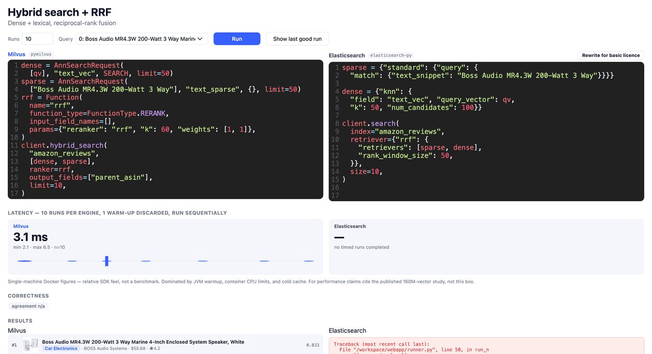
On a basic-licence Elasticsearch this returns a 403: rrf and linear are Platinum-tier retrievers, while Milvus's RRFRanker and WeightedRanker are in the free build. The free Elasticsearch path has to fuse knn and match with hand-tuned boost weights instead:
# Elasticsearch, basic-licence rewrite
client.search(
  index="amazon_reviews",
  query={"match": {"text_snippet": {
    "query": "wireless earbuds", "boost": 0.3}}},
  knn={
    "field": "text_vec", "query_vector": qv,
    "k": 50, "num_candidates": 100, "boost": 0.7,
  },
  size=10,
)
Those 0.3/0.7 weights are the real cost of combining two engines: BM25 scores are unbounded, cosine sits in 0–1, so you tune the weights by hand and re-tune them when the corpus moves. RRF avoids that by fusing on rank.
Grouping: group_by vs collapse
# Milvus
client.search(
  "amazon_reviews",
  data=[qv],
  anns_field="text_vec",
  group_by_field="main_category",
  group_size=1,
  search_params={"params": {"nprobe": 1, "rbq_bits_query": 4}},
  limit=10,
)
# Elasticsearch
client.search(
  index="amazon_reviews",
  knn={
    "field": "text_vec",
    "query_vector": qv,
    "k": 800,
    "num_candidates": 1600,
  },
  collapse={"field": "main_category.keyword"},
  size=10,
)
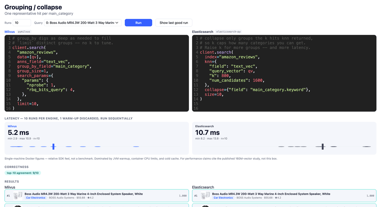
Milvus's group_by keeps reading until it fills limit distinct groups. Elasticsearch's collapse only groups the k hits kNN already returned, so k caps how many categories you get. To get more you raise k and pay for the larger scan regardless. That's k=800/num_candidates=1600 against limit=10: one is complete by construction, the other only if you over-fetch enough.
Server-side aggregation
Server-side aggregation is a new feature in Milvus 3.0, it's used by setting the field(s) to group by and defining the calculated fields in the output array:
# Milvus
client.query(
  "amazon_reviews",
  group_by_fields=["main_category"],
  output_fields=[
    "main_category", "count(*)", "avg(price)",
    "min(price)", "max(price)", "avg(average_rating)",
  ],
  order_by_fields=[{"field": "main_category", "order": "asc"}],
  limit=20,
)
Elasticsearch has had aggregations since version 1.0, it's used by setting your aggregation group and an object with the calculated output fields:
# Elasticsearch
client.search(
  index="amazon_reviews", size=0, request_cache=False,
  aggs={"by_group": {
    "terms": {
      "field": "main_category.keyword",
      "size": 20,
      "order": {"_key": "asc"},
    },
    "aggs": {
      "avg_price": {"avg": {"field": "price"}},
      "min_price": {"min": {"field": "price"}},
      "max_price": {"max": {"field": "price"}},
      "avg_rating": {"avg": {"field": "average_rating"}},
    },
  }},
)
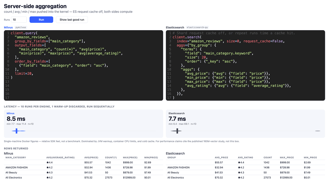
Both return the same aggregates, but Elasticsearch is slightly faster here (we've disabled the request cache for a pure aggregration performance test) - its terms aggregation is approximate when a field has more distinct values than each shard returns: shards send back only their local top terms, so counts can be underestimated and the top-N can be wrong. Milvus 3.0 computes aggregations exactly over all rows visible at query time. It returns every group. Aggregation in Milvus is new and still being optimised; if it’s central to your workload, benchmark it on your data and let us know which features you need.
Multi-stage reranking
Many search use cases require reranking and multiple stages, e.g. Initially fetching the most relevant results then reranking by ratings and finally by price. Multi-stage reranking is new in Milvus 3.0.1, and allows you to chain rerank functions to achieve complex business logic in a single search.
# Milvus
l0 = (FunctionChain(FunctionChainStage.L0_RERANK)
  .map("rated", fn.decay(col("average_rating"),
    function="linear", origin=5, scale=4))
  .map("$score", fn.num_combine(col("$score"), col("rated"),
    mode="weighted", weights=[1, 0.2])))
# L1 re-scores all 200 by price, keeps 50.
l1 = (FunctionChain(FunctionChainStage.L1_RERANK)
  .map("cheap", fn.decay(col("price"),
    function="gauss", origin=0, scale=30, offset=10))
  .map("$score", fn.num_combine(col("$score"), col("cheap"),
    mode="weighted", weights=[1, 0.2]))
  .sort("$score").limit(50))
# L2: 0.5 -> 1.0 ramp up to 100 reviews, keeps 10.
l2 = (FunctionChain(FunctionChainStage.L2_RERANK)
  .map("proven", fn.decay(col("rating_number"),
    function="linear", origin=1e6,
    offset=1e6 - 100, scale=100))
  .map("$score", fn.num_combine(col("$score"), col("proven"),
    mode="weighted", weights=[1, 0.2]))
  .sort("$score").limit(10))
client.search(
  "amazon_reviews",
  data=[qv],
  anns_field="text_vec",
  function_chains=[l0, l1, l2],
  limit=200,
)
The Elasticsearch syntax is an array of rescore functions:
# Elasticsearch
client.search(
  index="amazon_reviews",
  query={"function_score": {
    "query": {"knn": {
      "field": "text_vec", "query_vector": qv,
      "k": 200, "num_candidates": 400, "boost": 2}},
    "functions": [{"linear": {"average_rating": {
      "origin": 5, "scale": 4}}, "weight": 0.2}],
    "boost_mode": "sum",
  }},
  rescore=[
    {"window_size": 200, "query": {
      "rescore_query_weight": 0.2,
      "rescore_query": {"function_score": {"functions": [
        {"gauss": {"price": {
          "origin": 0, "scale": 30, "offset": 10}}}]}}}},
    {"window_size": 50, "query": {
      "rescore_query_weight": 0.2,
      "rescore_query": {"function_score": {"functions": [
        {"linear": {"rating_number": {"origin": 1e6,
          "offset": 1e6 - 100, "scale": 100}}}]}}}},
  ],
  size=10,
)
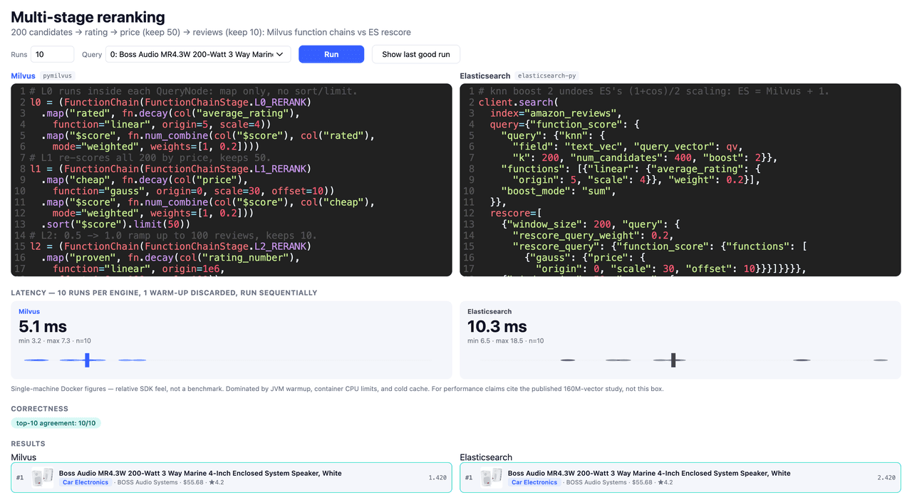
Quick summary of this comparison
Across the walkthrough, here's where each engine lands:
| Capability | Result |
|---|---|
| Dense (ANN) vector search | Tie: >0.99 recall@10 |
| Full-text (BM25) search | Tie: same top-10 |
| Hybrid search (RRF) | Milvus: one call, RRF in the free build; Elasticsearch gates it behind a paid tier |
| Grouping | Milvus: complete by construction; collapse is capped by k |
| Ordering, relevance shaping, geo, highlighting | Tie: same semantics, cleaner syntax |
| Memory footprint | Milvus: ~1.0 GB vs ~5 GB on the same data |
| Server-side aggregation | Elasticsearch: faster today; Milvus landed it in 3.0 and is tuning it |
| Multi-stage reranking | Tie: same top-10 |
| Typo-tolerant search | Elasticsearch today, on the Milvus roadmap |
Milvus matches Elasticsearch on the core keyword and vector operations, wins on hybrid search, grouping, and memory, and trails only on aggregation maturity and fuzzy matching which are both on the roadmap. For the workloads we see most commonly (keyword plus semantic search, increasingly for AI and RAG use cases), Milvus 3.0 covers both sides well enough to replace the two-engine stack at a smaller footprint. If your search is aggregation-first classic BM25, benchmark that path before you move; for everything hybrid or vector-heavy at scale, Milvus should be your first choice.
More is coming!
A few capabilities are still on the roadmap for future 3.x releases: typo-tolerant (fuzzy) search and search-as-you-type.
Fuzzy typos. Elasticsearch's edit-distance fuzziness catches user misspellings in searches. In Milvus 3.0, you can enumerate known misspellings in a synonym filter or use fuzzy match filtering, but true fuzzy BM25 search is coming soon.
Search-as-you-type. While there is not currently a phrase-prefix match query type in Milvus, you can achieve fast typeahead search by storing a normalized suggestion string for each entity / document, and add an NGRAM index to the field. You can then run LIKE "prefix%" queries with the normalised search characters and get a sub-5ms client-side response.
Interested? Read more here: https://simonhearne.com/2026/fast-typeahead-milvus/
Run the comparison yourself
docker compose up -d
python data/fetch.py        # one Parquet, ~370 MB
docker compose exec demo python data/load_milvus.py
docker compose exec demo python data/load_es.py
You'll want Docker with at least 16 GB of RAM. The code is at github.com/simonhearne/milvus_es_lab, with a walkthrough on YouTube. Load your own Parquet to run it on your data — that's the number that counts.
Teams that have already made the switch
Teams that ran two engines, hit one of these ceilings, and moved to a single engine on Milvus or Zilliz Cloud:
123RF (image search, OpenSearch → Zilliz Cloud): ~200M stock-asset vectors, search cost cut by more than half, latency halved to sub-50ms.
PLAUD (agent memory, OpenSearch → Zilliz Cloud): 10B+ memory chunks per region under 200ms average recall latency, across 2M+ devices.
Rexera (RAG + agents, Elasticsearch → Zilliz Cloud): hybrid search raised retrieval accuracy ~40% and cut cost ~50%.
Orfium (audio matching, Elasticsearch → Zilliz Cloud): ~250M audio vectors on Zilliz Cloud, well past the old setup's ceiling.
OpenArt (multimodal search, Elasticsearch → Zilliz Cloud): 456M vectors moved with no re-embedding; P99 from ~25s to ~300ms, compute cost down ~85%.
Figures from customer scenarios and internal testing; results vary with data scale, distribution, index parameters, and configuration. More: zilliz.com/customers.

Keep Reading
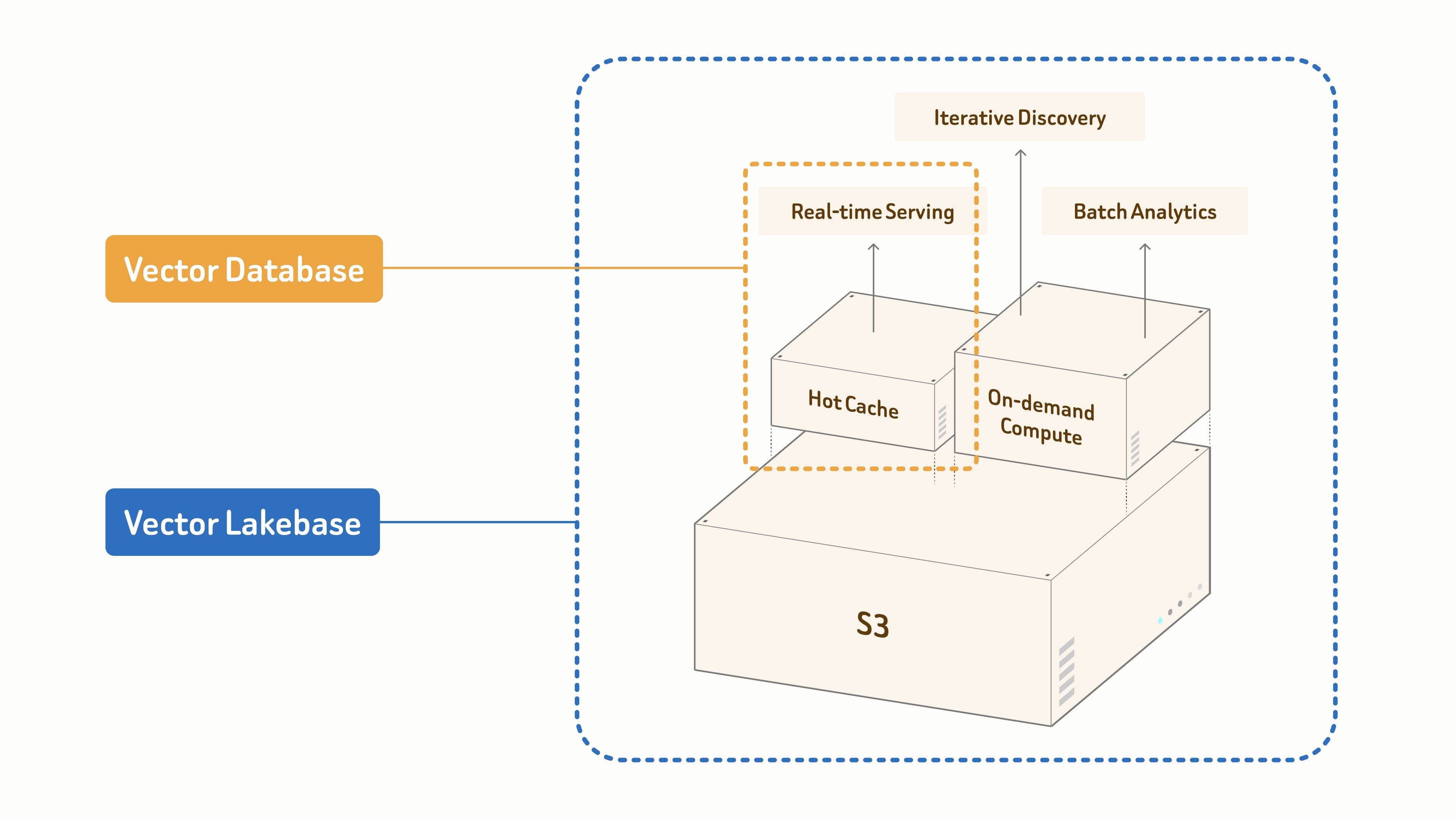
From Vector Database to Vector Lakebase
Zilliz offers a fully managed Vector Lakebase powered by Milvus, unifying real-time vector search, lake-scale discovery, and Al data operations.

How to Choose the Best Embedding Model for RAG in 2026: 10 Models Benchmarked
We benchmarked 10 embedding models on cross-modal, cross-lingual, long-document, and dimension compression tasks. See which one fits your RAG pipeline.

Democratizing AI: Making Vector Search Powerful and Affordable
Zilliz democratizes AI vector search with Milvus 2.6 and Zilliz Cloud for powerful, affordable scalability, cutting costs in infrastructure, operations, and development.