Blog
Visualize Reverse Image Search with Feder

Visualize Reverse Image Search with Feder

May 25, 20226 min read

Reverse image search is one the most prevalent applications of vector search or approximate nearest neighbor search. When a user uploads an image to the search engine, a bunch of similar images will be returned. During the process, indexes are built to accelerate the search on large datasets, especially those billion- or even trillion-scale datasets.

In the previous blog, we have introduced how to visualize your approximate nearest neighbor search with Feder by using the example of HNSW index visualization. In this article, we will take the example of reverse image search and continue to explain how you can use Feder to visualize the index building and search process. In this article, we use the IVF_FLAT index as it is the most commonly used index in reverse image search applications.

How to visualize reverse image search with Feder

Feder is built with JavaScript. To use Feder for visualization, you need to first build an index and save the index file from Faiss or Hnswlib. Then Feder analyzes the uploaded file to obtain index information and gets ready for the visualization. During a vector similarity search, you need to provide a target vector and the configuration of search parameters. Then Feder visualizes the whole search process for you.

Learn more about how to use Feder by reading Feder user guide.

A use case of visualizing search with IVF_FLAT index

In this use case, we use VOC 2012, the classic ML image dataset that contains more than 17,000 images.

First, we use Towhee, an open-source ML pipeline to encode the images in the VOC 2012 dataset into vectors. Then we build an IVF_FLAT index with Faiss and save the index file. Finally, use Feder for visualization.

Build an IVF_Flat index

Indexes are built to accelerate the search process. An analogy can be drawn to a dictionary. All of the words are organized based on their initials. More specifically, words with the same initials are grouped together. And we all know that the number of entries under each initial is unequal. We have more words starting with the letter "E" than those starting with "Z". When looking up a word, we can quickly navigate to the section that only contains words with the same initial. This helps drastically boost the search speed.

Similarly, the IVF_FLAT index divides vectors in the vector space into different clusters based on vector distance. Vectors close to each other are more likely to be put in the same cluster. And the vectors are not necessarily evenly distributed in each cluster. Therefore, each cluster contains a different amount of vectors.

In this use case, we used Faiss to build an IVF_FLAT index on the 17,000 images in the VOC 2012 dataset, with an nlist of 256. The 17,000 image vectors are divided into 256 clusters based on K-means clustering method.

With Feder, you can visualize the clustering of high-dimensional vector space in a 2D view. Feder supports viewing the details of each cluster while providing an interactive user experience. To have a better understanding of the IVF_FLAT index, you can click on one of the clusters in Feder, and then you will see a maximum of nine images represented by vectors within this cluster.

Coarse search

When you input a target image and convert it into a target vector for reverse image search, the system first calculates the distance between the target vector and the centroid of each cluster to find the nearest clusters.

In this use case, nlist equals 256, which means that the whole vector space is divided into 265 cluster units. Therefore, in the coarse search process, the system compares the distance between the target vector and 256 cluster centroids.

In IVF indexes, the vectors are clustered based on their relative distance to each other. This means that it is highly likely that the nearest neighbors of the target vector is located in its nearest clusters. We can control the number of cluster units to query with the parameter nprobe. In this use case, nprobe equals 8 meaning that the system will look for the nearest neighbor of the target vector within the top eight closest clusters.

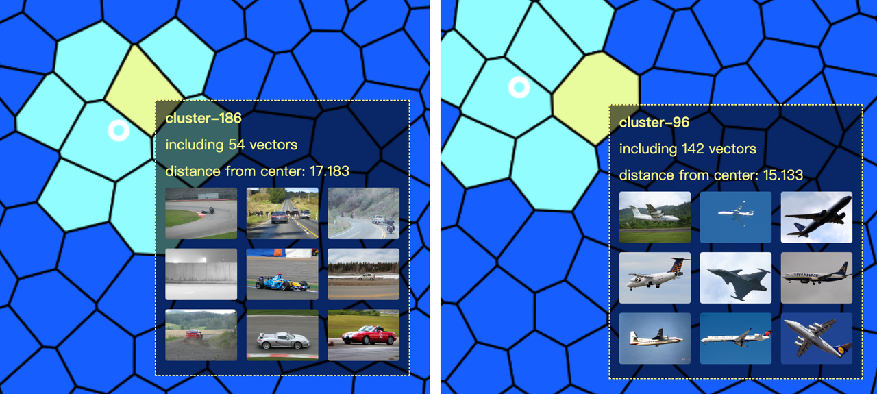
The screenshot below is a detailed view of the closest clusters. In cluster-186 (the eighth closest cluster to the target vector) we can see it contains some vectors of car images. Though the cars are not at all similar to the airplane in our target image, the images in cluster-186 and the target do share some resemblance as the car tracks in cluster-186 images look very much alike the airport runway in the target image. In a much closer cluster, cluster-96, we can see it contains images of aircrafts in the sky.

Coarse search.

The clusters in this use case demonstrate that during embedding, the machine learning model accurately extracts the features including aircraft, runway, and sky in the target image. Then it divides vectors in the vector space based on these features. Cluster-186 shares the feature of "runway" while cluster-96 shares the feature of "aircraft".

Fine search

After a coarse search, we can secure a number of nprobe clusters for a fine search. In this stage, the system compares the distance between the target vector and all vectors in the nprobe clusters. Then the topK closest vectors are returned as the final results.

In this use case, the system calculates the distance between the target vector and a total of 742 vectors in 8 clusters during the fine search process.

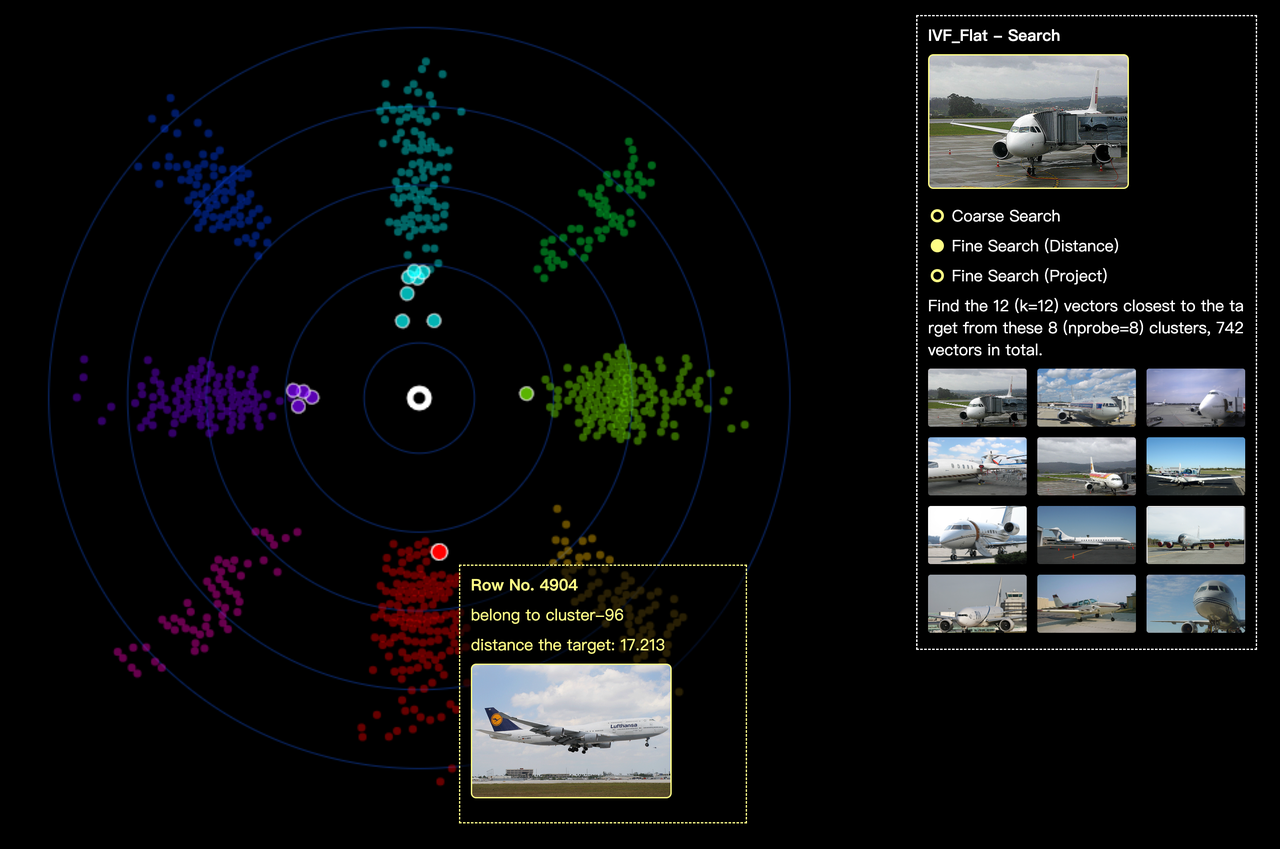
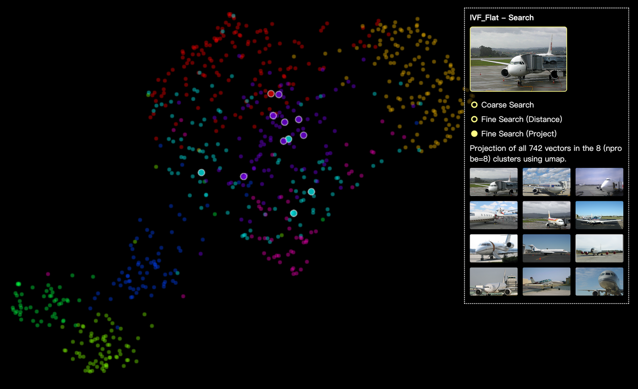
Feder provides two visualization modes for the fine search process. One mode is visualization based on cluster and vector distance. The other is the projection for dimension reduction mode.

In the screenshot below, different clusters are shown in different colors. The white circle in the center represents the target vector. With the help of Feder, you can see the distance between each vector and the target vector in a clearer and more straight-forward way. You can click on each vector to see more detailed information like its distance to target vector, the image it represents, etc.

Fine search.

The screenshot below is the projection for dimension reduction mode. Still, different clusters are shown in different colors. Currently, we only support UMAP, one of the most popular method for dimension reduction. More project methods will be supported in future releases of Feder.

Fine search.

Search performance analysis

When searching without an index, the system needs to calculate the distance between the target vector and all the 17,000 vectors in the database. However, by contrast, if we build an IVF_FLAT index, search efficiency is greatly boosted as the calculation volume is significantly reduced (the system only need to calculate the distance between the target vector and the 256 cluster centroids in coarse search and 742 vectors in fine search).

Also with Feder visualization, we will realize that the value of the index building parameters will influence how the vector space is divided. The nprobe parameter can be used to achieve tradeoff between search efficiency and accuracy. The higher the value of nprobe, the broader the search scope, and the more accurate the results are. But accordingly, search efficiency will be compromised as the calculation volume increases.