



Milvus 2.1을 사용한 ArXiv 과학 논문 벡터 유사도 검색
소개
최신 데이터 과학 주제를 배우는 가장 좋은 방법 중 하나는 arxiv.org에서 오픈 소스 연구 논문을 읽는 것입니다. 그러나 방대한 수의 연구 논문은 가장 노련한 연구자에게도 훑어보고 정리하기에 압도적일 수 있습니다. connected papers와 같은 도구가 도움이 될 수 있지만, 이러한 도구는 문서 내 텍스트의 의미적 의미가 아니라 논문 간에 공유되는 인용 및 참고문헌을 기반으로 유사성을 측정합니다.
이 글에서는 하나의 “쿼리” 논문을 입력으로 받아 최첨단 NLP를 사용해 약 64만 편의 컴퓨터 과학 논문으로 구성된 arxiv 코퍼스에서 가장 유사한 상위 K개 논문을 찾는 의미적 유사도 검색 엔진을 구축해 보겠습니다! 검색은 단일 노트북에서 <50ms 지연 시간으로 실행됩니다! 구체적으로 이 글에서는 다음을 다룹니다
- 환경을 설정하고 Kaggle에서 arXiv 데이터를 다운로드하기
- Dask를 사용해 데이터를 Python으로 로드하기
- Milvus 벡터 데이터베이스를 사용해 과학 논문 의미적 유사도 검색 애플리케이션 구현하기
이 글에서 사용한 기법은 과학 논문뿐만 아니라 어떤 NLP 의미적 유사도 검색 엔진을 구축하는 데에도 템플릿으로 사용할 수 있습니다. 유일한 차이는 사용되는 사전 학습 모델입니다.
이 글에서는 저자들이 CC0: Public Domain 라이선스로 공개한 Kaggle의 arXiv Dataset을 사용하겠습니다.
저는 이전 글에서 프로덕션 규모의 벡터 유사도 검색 고려사항을 정리했습니다. 이러한 모든 고려사항은 이 프로젝트에도 적용됩니다. Milvus 벡터 데이터베이스는 매우 잘 설계되어 있어 많은 단계가 정확히 동일하며, 여기서는 완전성을 위해서만 다시 포함했습니다.
환경을 설정하고 Kaggle에서 arxiv 데이터를 다운로드하기.
Cornel University는 전체 arXiv 코퍼스를 Kaggle dataset에 업로드하고 CC0: Public Domain 라이선스로 제공했습니다. Kaggle API를 사용해 데이터셋을 직접 다운로드할 수 있습니다. 아직 하지 않았다면 이 지침을 따라 시스템에 Kaggle API를 설정하세요.
이 글에서는 semantic_similarity라는 conda 환경을 사용하겠습니다. 시스템에 conda를 설치하지 않았다면 해당 GitHub repository에서 오픈 소스 mini forge를 설치하여 사용할 수 있습니다. 아래 단계는 필요한 디렉터리와 conda 환경을 만들고, 필요한 Python 라이브러리를 설치하며, Kaggle의 arxiv dataset을 다운로드합니다.
# Create the necessary directories
mkdir -p semantic_similarity/notebooks semantic_similarity/data semantic_similarity/milvus

# CD into the data directory
cd semantic_similarity/data

# Create and activate a conda environment
conda create -n semantic_similarity python=3.9
conda activate semantic_similarity

## Create Virtual Environment using venv if not using conda
# python -m venv semantic_similarity
# source semantic_similarity/bin/activate

# Pip install the necessary libraries
pip install jupyterlab kaggle matplotlib scikit-learn tqdm ipywidgets
pip install "dask[complete]" sentence-transformers
pip install pandas pyarrow pymilvus protobuf==3.20.0

# Download data using the kaggle API
kaggle datasets download -d Cornell-University/arxiv

# Unzip the data into the local directory
unzip arxiv.zip

# Delete the Zip file
rm arxiv.zip
Dask를 사용해 데이터를 Python으로 로드하기
Kaggle에서 다운로드한 데이터는 약 200만 편의 논문을 포함하는 3.3GB JSON 파일입니다! 이렇게 큰 데이터셋을 효율적으로 처리하려면 pandas를 사용해 전체 데이터셋을 메모리에 로드하는 것은 좋은 생각이 아닙니다. 대신 Dask를 사용해 데이터를 여러 파티션으로 나누고, 특정 시점에는 몇 개의 파티션만 메모리에 로드할 수 있습니다.
Dask
Dask는 pandas와 유사한 API로 병렬 컴퓨팅을 쉽게 적용할 수 있게 해주는 오픈소스 라이브러리입니다. 설정 섹션에 표시된 것처럼 pip install dask[complete]를 실행하면 로컬 머신에서 간단히 설정할 수 있습니다. 먼저 필요한 라이브러리들을 임포트하는 것부터 시작해 보겠습니다.
import dask.bag as db
import json
from datetime import datetime
import time

data_path = '../data/arxiv-metadata-oai-snapshot.json'
큰 arxiv JSON 파일을 효율적으로 처리하기 위해 Dask의 두 가지 구성 요소를 사용하겠습니다.
- Dask Bag: JSON 파일을 고정된 크기의 블록으로 로드하고 각 데이터 행에 일부 전처리 함수를 실행할 수 있게 해줍니다.
- Dask DataFrame: dask bag을 dask dataframe으로 변환하여 pandas와 유사한 API에 접근할 수 있습니다
Step 1: JSON 파일을 Dask bag으로 로드하기
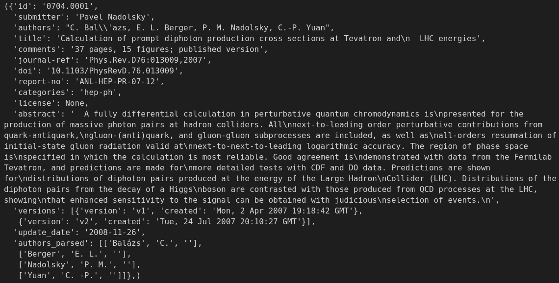
JSON 파일을 각 블록 크기가 10MB인 dask bag으로 로드해 보겠습니다. blocksize 인수를 조정하여 각 블록의 크기를 원하는 대로 제어할 수 있습니다. 그런 다음 .map() 함수를 사용해 dask bag의 모든 행에 json.loads 함수를 적용하여 JSON 문자열을 Python 딕셔너리로 파싱합니다.
# Read the file in blocks of 10MB and parse the JSON.
papers_db = db.read_text(data_path, blocksize="10MB").map(json.loads)

# Print the first row
papers_db.take(1)
 저자 제공 이미지
Step 2: 전처리 헬퍼 함수 작성하기
출력 결과를 보면 각 행에 논문과 관련된 여러 메타데이터가 포함되어 있음을 알 수 있습니다. 데이터셋을 전처리하는 데 도움이 되도록 세 가지 헬퍼 함수를 작성해 보겠습니다.
v1_date(): 이 함수는 저자들이 논문의 첫 번째 버전을 arXiv에 업로드한 날짜를 추출합니다. 날짜를 UNIX 시간으로 변환하여 해당 행의 새 필드로 저장하겠습니다.text_col(): 이 함수는 “title” 및 “abstract” 필드를 “[SEP]” 토큰으로 결합하여 이 텍스트들을 SPECTRE embedding model에 입력할 수 있게 합니다. SPECTRE에 대해서는 다음 섹션에서 더 이야기하겠습니다.filters(): 이 함수는 여러 열의 최대 텍스트 길이 및 Computer Science 카테고리의 논문과 같은 몇 가지 기준을 충족하는 행만 유지합니다.
def v1_date(row):
    """
    For each row in the dask bag,
    find the date of the first version of the paper
    and add it to the row as a new column
    Args:
      row: a row of the dask bag
    Returns:
      A row of the dask bag with added "unix_time" column
    """

    versions = row["versions"]

    date = None
    for version in versions:
        if version["version"] == "v1":
            date = datetime.strptime(version["created"], "%a, %d %b %Y %H:%M:%S %Z")
            date = int(time.mktime(date.timetuple()))

    row["unix_time"] = date

    return row

def text_col(row):
    """
    It takes a row of a dataframe, adds a new column called 'text'
    that is the concatenation of the 'title' and 'abstract' columns
    Args:
      row: the row of the dataframe
    Returns:
      A row with the text column added.
    """

    row["text"] = row["title"] + "[SEP]" + row["abstract"]
    return row

def filters(row):
    """
    For each row in the dask bag, only keep the row if it meets the filter criteria

    Args:
      row: the row of the dataframe
    Returns:
      Boolean mask
    """

    return ((len(row["id"])<16) and
            (len(row["categories"])<200) and
            (len(row["title"])<4096) and
            (len(row["abstract"])<65535) and
            ("cs." in row["categories"]) # Keep only CS papers
           )
3단계: Dask bag에서 전처리 헬퍼 함수 실행하기
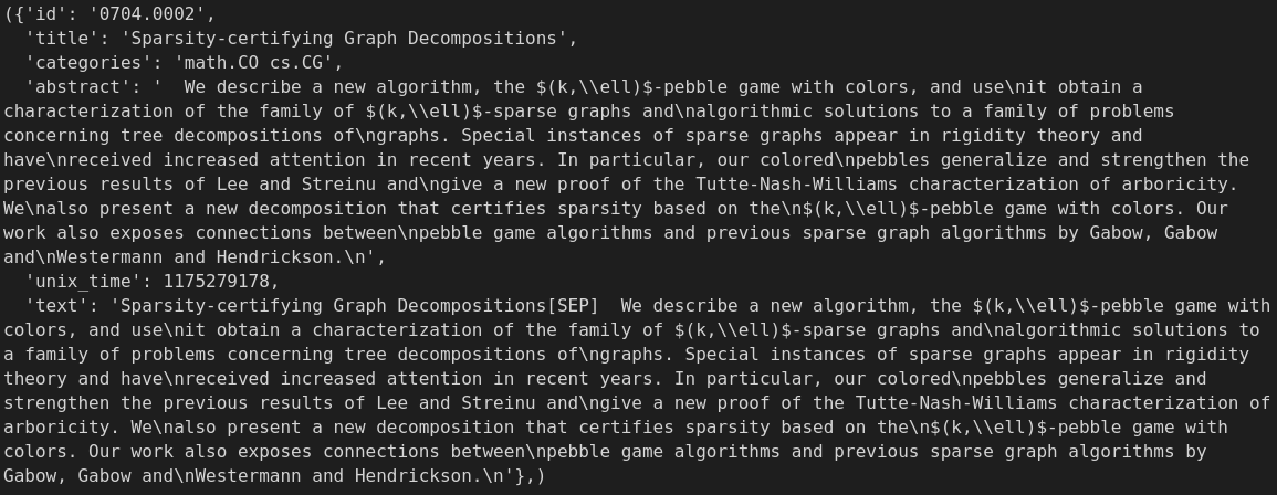
아래와 같이 .map() 및 .filter() 함수를 사용하여 Dask bag의 모든 행에서 헬퍼 함수를 쉽게 실행할 수 있습니다. Dask는 메서드 체이닝을 지원하므로, 이 기회를 활용해 Dask bag에서 몇 가지 필수 열만 유지하고 나머지는 삭제합니다.
# Specify columns to keep in the final table
cols_to_keep = ["id", "categories", "title", "abstract", "unix_time", "text"]

# Apply the pre-processing
papers_db = (
    papers_db.map(lambda row: v1_date(row))
    .map(lambda row: text_col(row))
    .map(
        lambda row: {
            key: value
            for key, value in row.items()
            if key in cols_to_keep
        }
    )
    .filter(filters)
)

# Print the first row
papers_db.take(1)
 저자 제공 이미지
4단계: Dask Bag을 Dask DataFrame으로 변환하기
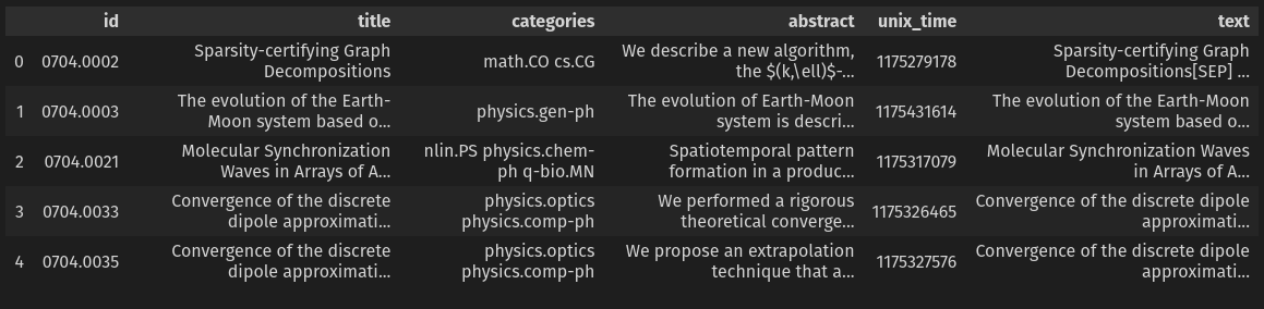
데이터 로딩의 마지막 단계는 Dask Bag을 Dask Dataframe으로 변환하여 데이터의 각 블록 또는 파티션에서 pandas와 유사한 API를 사용하는 것입니다.
# Convert the Dask Bag to a Dask Dataframe
schema = {
    "id": str,
    "title": str,
    "categories": str,
    "abstract": str,
    "unix_time": int,
    "text": str,
}
papers_df = papers_db.to_dataframe(meta=schema)

# Display first 5 rows
papers_df.head()
 저자 제공 이미지
Milvus 벡터 데이터베이스를 사용한 과학 논문 의미적 유사도 검색 애플리케이션 구현하기
Milvus는 확장성이 매우 뛰어나고 매우 빠른 유사도 검색을 위해 구축된 가장 인기 있는 오픈 소스 벡터 데이터베이스 중 하나입니다. 이 글에서는 로컬 머신에서만 Milvus를 실행하므로 Milvus Standalone을 사용하겠습니다.
1단계: 로컬에 Milvus 벡터 데이터베이스 설치하기
Milvus 벡터 데이터베이스는 Docker를 사용하면 매우 쉽게 설치할 수 있으므로 먼저 Docker와 Docker Compose를 설치해야 합니다. 그런 다음 아래 코드 스니펫에 표시된 것처럼 docker-compose.yml을 다운로드하고 docker 컨테이너를 시작하기만 하면 됩니다! milvus.io 웹사이트는 Milvus standalone과 Milvus Cluster를 모두 설치할 수 있는 여러 다른 옵션을 제공합니다. Kubernetes 클러스터에 설치하거나 오프라인으로 설치해야 하는 경우 확인해 보세요.
# CD into milvus directory
cd semantic_similarity/milvus

# Download the Standalone version of Milvus docker compose
wget https://github.com/milvus-io/milvus/releases/download/v2.1.0/milvus-standalone-docker-compose.yml -O ./docker-compose.yml

# Run the Milvus server docker container on your local
sudo docker-compose up -d
2단계: Milvus 컬렉션 생성하기
이제 로컬 머신에서 Milvus 벡터 데이터베이스 서버가 실행 중이므로, pymilvus 라이브러리를 사용하여 상호작용할 수 있습니다. 먼저 필요한 모듈을 가져오고 localhost에서 실행 중인 Milvus 서버에 연결해 보겠습니다. alias 및 collection_name 매개변수는 자유롭게 변경해도 됩니다. 텍스트를 임베딩으로 변환하는 데 사용하는 모델이 emb_dim 매개변수의 값을 결정합니다. SPECTRE의 경우 임베딩은 768d입니다.
# Milvus 서버가 이미 실행 중인지 확인하세요
from pymilvus import connections, utility
from pymilvus import Collection, CollectionSchema, FieldSchema, DataType

# Milvus 서버에 연결
connections.connect(alias="default", host="localhost", port="19530")

# 컬렉션 이름
collection_name = "arxiv"

# 임베딩 크기
emb_dim = 768

# # 기존 컬렉션을 확인하고 존재하면 삭제
# if utility.has_collection(collection_name):
#     print(utility.list_collections())
#     utility.drop_collection(collection_name)
선택적으로, collection_name으로 지정된 컬렉션이 Milvus 서버에 이미 존재하는지 확인할 수 있습니다. 이 예제에서는 컬렉션이 이미 있으면 삭제합니다. 하지만 프로덕션 서버에서는 이렇게 하지 않고, 대신 아래의 컬렉션 생성 코드를 건너뛰게 됩니다.
Milvus 컬렉션은 전통적인 데이터베이스의 테이블과 유사합니다. 데이터를 저장할 컬렉션을 만들려면 먼저 컬렉션의 schema를 지정해야 합니다. 이 예제에서는 각 논문과 관련된 모든 필수 메타데이터를 저장하기 위해 문자열 인덱스와 필드를 저장할 수 있는 Milvus 2.1의 기능을 활용합니다. 기본 키 idx와 기타 필드 categories, title, abstract는 적절한 최대 길이를 가진 VARCHAR 데이터 타입을 가지며, embedding은 emb_dim 차원 임베딩을 포함하는 FLOAT_VECTOR필드입니다. Milvus는 문서 페이지에 표시된 것처럼 다양한 데이터 타입을 지원합니다.
# 컬렉션에 대한 스키마 생성
idx = FieldSchema(name="id", dtype=DataType.VARCHAR, is_primary=True, max_length=16)
categories = FieldSchema(name="categories", dtype=DataType.VARCHAR, max_length=200)
title = FieldSchema(name="title", dtype=DataType.VARCHAR, max_length=4096)
abstract = FieldSchema(name="abstract", dtype=DataType.VARCHAR, max_length=65535)
unix_time = FieldSchema(name="unix_time", dtype=DataType.INT64)
embedding = FieldSchema(name="embedding", dtype=DataType.FLOAT_VECTOR, dim=emb_dim)

# 컬렉션의 필드
fields = [idx, categories, title, abstract, unix_time, embedding]
schema = CollectionSchema(
    fields=fields, description="Semantic Similarity of Scientific Papers"
)

# 스키마로 컬렉션 생성
collection = Collection(
    name=collection_name, schema=schema, using="default", shards_num=10
)
컬렉션이 생성되면, 이제 텍스트와 벡터를 그 안에 업로드할 준비가 된 것입니다.
3단계: Dask 데이터프레임의 파티션을 반복하며, SPECTER를 사용해 텍스트를 임베딩하고, Milvus 벡터 데이터베이스에 업로드하기
먼저 의미적 유사도 검색을 실행하기 위해 Dask 데이터프레임의 텍스트를 임베딩 벡터로 변환해야 합니다. 아래 제 게시물에서는 텍스트를 임베딩으로 변환하는 방법을 공유합니다. 특히, 과학 논문을 임베딩으로 변환하기 위해 SPECTRE라는 SBERT Bi-Encoder 모델을 사용할 것입니다.
SPECTER [논문] [Github]: Scientific Paper Embeddings using Citation-informed TransformERs는 과학 논문을 임베딩으로 변환하는 모델입니다.
- 각 논문의 Title 및 Abstract 텍스트는 [SEP] 토큰으로 연결되고 사전 학습된 Transformer 모델(SciBERT)의 [CLS] 토큰을 사용해 임베딩으로 변환됩니다.
- 인용을 문서 간 관련성의 대리 신호로 사용합니다. 한 논문이 다른 논문을 인용한다면, 두 논문이 서로 관련되어 있다고 추론할 수 있습니다.
- Triplet loss 학습 목표: 우리는 Transformer 모델을 학습시켜, 인용을 공유하는 논문들이 임베딩 공간에서 더 가깝도록 합니다.
- 다시 말해, Positive 논문은 Query 논문에서 인용된 논문이고, Negative 논문은 Query 논문에서 인용되지 않은 논문입니다. 무작위로 샘플링된 negatives는 “easy” negatives입니다.
- 성능을 향상시키기 위해, Query 논문에서는 인용되지 않았지만 Positive 논문에서는 인용된 논문을 사용하여 “hard” negatives를 만듭니다.
- 추론 시에는 Title과 Abstract만 필요합니다. 인용은 필요하지 않으므로, SPECTER는 아직 인용이 전혀 없는 새로운 논문에 대해서도 임베딩을 생성할 수 있습니다!
- SPECTER는 주제 분류, 인용 예측, Scientific Papers 추천에서 뛰어난 성능(SciBERT보다 우수)을 제공합니다.
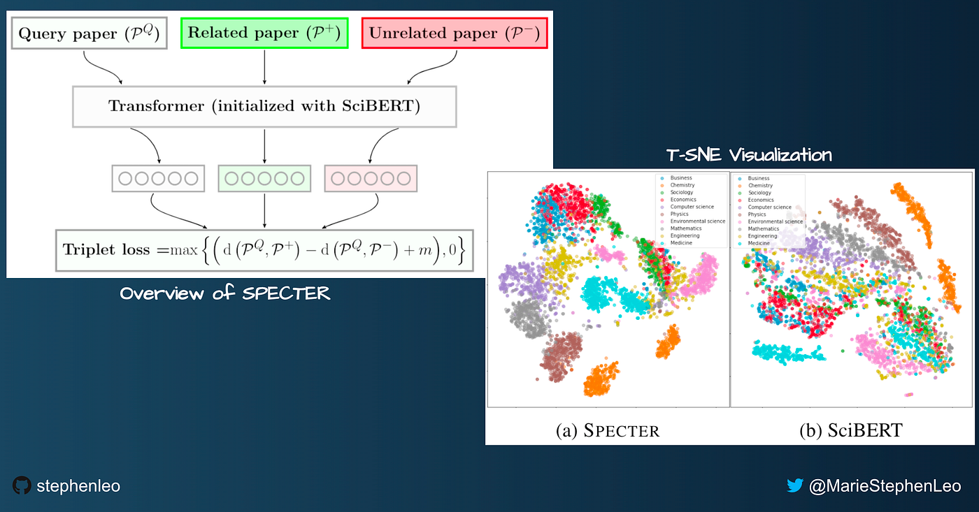 스크린샷을 사용하여 저자가 만든 이미지, 오픈소스 SPECTER 논문 출처
사전 학습된 SPECTRE 모델을 사용하는 것은 Sentence Transformer 라이브러리를 사용하면 간단합니다. 아래에 보이는 것처럼 단 한 줄의 코드로 사전 학습된 모델을 다운로드할 수 있습니다. 또한 Dask dataframe 파티션의 텍스트 전체 열을 임베딩으로 변환하는 간단한 헬퍼 함수도 작성합니다.
from sentence_transformers import SentenceTransformer
from tqdm import tqdm

# Scientific Papers SBERT Model
model = SentenceTransformer('allenai-specter')

def emb_gen(partition):
    return model.encode(partition['text']).tolist()
데이터를 Milvus collection에 업로드하기 위해 Dask dataframe의 파티션을 반복해야 합니다. 각 반복에서 해당 파티션의 행만 메모리에 로드하고 metadata 열의 데이터를 data 변수에 추가합니다. dask .map_partitions() API를 사용하여 파티션의 모든 행에 임베딩 생성을 적용하고 결과를 동일한 data 변수에 다시 추가할 수 있습니다. 마지막으로 collection.insert로 데이터를 Milvus에 업로드할 수 있습니다.
# Initialize
collection = Collection(collection_name)

for partition in tqdm(range(papers_df.npartitions)):
    # Get the dask dataframe for the partition
    subset_df = papers_df.get_partition(partition)

    # Check if dataframe is empty
    if len(subset_df.index) != 0:
        # Metadata
        data = [
            subset_df[col].values.compute().tolist()
            for col in ["id", "categories", "title", "abstract", "unix_time"]
        ]

        # Embeddings
        data += [
            subset_df
            .map_partitions(emb_gen)
            .compute()[0]
        ]

        # Insert data
        collection.insert(data)
data 변수에 추가되는 열의 순서는 스키마 생성 중에 정의한 fields 변수와 동일한 순서를 따라야 한다는 점에 유의하세요!
Step 4: 업로드된 데이터에 Approximate Nearest Neighbors (ANN) index 생성하기
모든 임베딩을 Milvus vector database에 삽입한 후에는 검색 속도를 높이기 위해 ANN index를 생성해야 합니다. 이 예시에서는 HNSW index type, 즉 가장 빠르고 정확한 ANN indexes 중 하나를 사용합니다. HNSW index와 그 매개변수에 대한 자세한 정보는 Milvus documentation을 참고하세요.
# Add an ANN index to the collection
index_params = {
    "metric_type": "L2",
    "index_type": "HNSW",
    "params": {"efConstruction": 128, "M": 8},
}

collection.create_index(field_name="embedding", index_params=index_params)
Step 5: Vector Similarity Search 쿼리 실행하기!
마침내 Milvus 컬렉션의 데이터를 쿼리할 준비가 되었습니다. 먼저, 컬렉션에 대해 쿼리를 실행하려면 컬렉션을 메모리에 로드해야 합니다.
# Load the collection into memory
collection = Collection(collection_name)
collection.load()
다음으로, query_text를 입력받아 SPECTRE 임베딩으로 변환하고, Milvus 컬렉션 전체에서 ANN 검색을 실행한 뒤 결과를 출력하는 간단한 헬퍼 함수를 만들었습니다. HNSW 문서 페이지에 설명된 search_params를 사용해 검색 품질과 속도를 제어할 수 있습니다.
def query_and_display(query_text, collection, num_results=10):
    # Embed the Query Text
    query_emb = [model.encode(query_text)]

    # Search Params
    search_params = {"metric_type": "L2", "params": {"ef": 128}}

    # Search
    query_start = datetime.now()
    results = collection.search(
        data=query_emb,
        anns_field="embedding",
        param=search_params,
        limit=num_results,
        expr=None,
        output_fields=["title", "abstract"],
    )
    query_end = datetime.now()

    # Print Results
    print(f"Query Speed: {(query_end - query_start).total_seconds():.2f} s")
    print("Results:")
    for res in results[0]:
        title = res.entity.get("title").replace("\n ", "")
        print(f"➡️ ID: {res.id}. L2 Distance: {res.distance:.2f}")
        print(f"Title: {title}")
        print(f"Abstract: {res.entity.get('abstract')}")
이제 단 한 줄의 코드로 헬퍼 함수를 사용하여 Milvus 컬렉션에 저장된 전체 약 64만 편의 Computer Science 논문을 대상으로 의미 기반 arXiv 논문 검색을 실행할 수 있습니다. 예를 들어, 저는 이전 게시물에서 자세히 다룬 SimCSE 논문과 유사한 논문들을 검색하고 있습니다. 상위 10개 결과는 대부분 문장 임베딩의 대조 학습과 관련되어 있어 제 검색 쿼리와 상당히 관련성이 높습니다! 전체 검색이 제 노트북에서 실행했을 뿐인데도 30ms밖에 걸리지 않았다는 점은 더욱 인상적이며, 이는 대부분의 애플리케이션에서 일반적인 사용 요구 사항을 충분히 충족하는 수준입니다!
# Query for papers that are similar to the SimCSE paper
title = "SimCSE: Simple Contrastive Learning of Sentence Embeddings"
abstract = """This paper presents SimCSE, a simple contrastive learning framework that greatly advances state-of-the-art sentence embeddings. We first describe an unsupervised approach, which takes an input sentence and predicts itself in a contrastive objective, with only standard dropout used as noise. This simple method works surprisingly well, performing on par with previous supervised counterparts. We find that dropout acts as minimal data augmentation, and removing it leads to a representation collapse. Then, we propose a supervised approach, which incorporates annotated pairs from natural language inference datasets into our contrastive learning framework by using "entailment" pairs as positives and "contradiction" pairs as hard negatives. We evaluate SimCSE on standard semantic textual similarity (STS) tasks, and our unsupervised and supervised models using BERT base achieve an average of 76.3% and 81.6% Spearman's correlation respectively, a 4.2% and 2.2% improvement compared to the previous best results. We also show -- both theoretically and empirically -- that the contrastive learning objective regularizes pre-trained embeddings' anisotropic space to be more uniform, and it better aligns positive pairs when supervised signals are available."""

query_text = f"{title}[SEP]{abstract}"
query_and_display(query_text, collection, num_results=10)
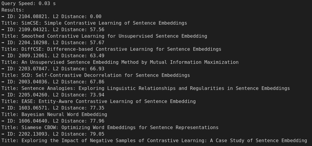 저자 제공 이미지
더 이상 쿼리를 실행할 필요가 없다면, 머신의 메모리를 확보하기 위해 컬렉션을 해제할 수 있습니다. 컬렉션을 메모리에서 제거해도 데이터 손실은 발생하지 않습니다. 데이터는 여전히 디스크에 저장되어 있으며 필요할 때 다시 로드할 수 있기 때문입니다.
# Release the collection from memory when it's not needed anymore
collection.release()
Milvus 서버를 중지하고 디스크에서 모든 데이터를 삭제하려면 Milvus 중지 지침을 따르면 됩니다. 주의하세요! 이 작업은 되돌릴 수 없으며 Milvus 클러스터의 모든 데이터를 삭제합니다.
결론
이 게시물에서는 SPECTRE 임베딩과 Milvus 벡터 데이터베이스를 사용하여 몇 가지 쉬운 단계만으로 초확장형 과학 논문 시맨틱 검색 서비스를 구현했습니다. 이 접근 방식은 프로덕션에서 수억 또는 심지어 수십억 개의 벡터까지 확장 가능합니다. 샘플 논문 쿼리를 사용해 검색을 테스트했으며, 단 30ms 만에 상위 10개 결과를 반환했습니다! 고도로 확장 가능하고 매우 빠른 벡터 유사도 검색 데이터베이스라는 Milvus의 평판은 충분히 그럴 만합니다!
Milvus 애플리케이션에 대한 더 많은 영감을 얻으려면 Milvus 벡터 데이터베이스 데모와 Bootcamp를 확인해 주세요.

계속 읽기
My Wife Wanted Dior. I Spent $600 on Claude Code to Vibe-Code a 2M-Line Database Instead.
Write tests, not code reviews. How a test-first workflow with 6 parallel Claude Code sessions turns a 2M-line C++ codebase into a daily shipping pipeline.
Zilliz Cloud BYOC Now Available Across AWS, GCP, and Azure
Zilliz Cloud BYOC is now generally available on all three major clouds. Deploy fully managed vector search in your own AWS, GCP, or Azure account — your data never leaves your VPC.

How to Use Anthropic MCP Server with Milvus
MCP + Milvus: Streamline AI agent development with standardized data access, eliminating integration hassles while enhancing context and flexibility.